🎲 Samples, Populations, Statistics and Inference

Sampling

Central Limit Theorem

Standard Error

Confidence Intervals

Published

November 25, 2022

Modified

March 1, 2025

Abstract

How much ~~Land~~ Data does a Man need?

Slides and Tutorials

R Tutorial

Datasets

“When Alexander the Great visited Diogenes and asked whether he could do anything for the famed teacher, Diogenes replied:”Only stand out of my light.” Perhaps some day we shall know how to heighten creativity. Until then, one of the best things we can do for creative men and women is to stand out of their light.”

— John W. Gardner, author and educator (8 Oct 1912-2002)

Setting up R Packages

library(tidyverse) # Data Processing in R
library(mosaic) # Our workhorse for stats, sampling
library(skimr) # Good to Examine data
library(ggformula) # Formula interface for graphs

# load the NHANES data library
library(NHANES)
library(infer)

Plot Theme

Show the Code

# https://stackoverflow.com/questions/74491138/ggplot-custom-fonts-not-working-in-quarto

# Chunk options
knitr::opts_chunk$set(
  fig.width = 7,
  fig.asp = 0.618, # Golden Ratio
  # out.width = "80%",
  fig.align = "center"
)
### Ggplot Theme
### https://rpubs.com/mclaire19/ggplot2-custom-themes

theme_custom <- function() {
  font <- "Roboto Condensed" # assign font family up front

  theme_classic(base_size = 14) %+replace% # replace elements we want to change

    theme(
      panel.grid.minor = element_blank(), # strip minor gridlines
      text = element_text(family = font),
      # text elements
      plot.title = element_text( # title
        family = font, # set font family
        # size = 20,               #set font size
        face = "bold", # bold typeface
        hjust = 0, # left align
        # vjust = 2                #raise slightly
        margin = margin(0, 0, 10, 0)
      ),
      plot.subtitle = element_text( # subtitle
        family = font, # font family
        # size = 14,                #font size
        hjust = 0,
        margin = margin(2, 0, 5, 0)
      ),
      plot.caption = element_text( # caption
        family = font, # font family
        size = 8, # font size
        hjust = 1
      ), # right align

      axis.title = element_text( # axis titles
        family = font, # font family
        size = 10 # font size
      ),
      axis.text = element_text( # axis text
        family = font, # axis family
        size = 8
      ) # font size
    )
}

# Set graph theme
theme_set(new = theme_custom())
#

What is a Population?

A population is a collection of individuals or observations we are interested in. This is also commonly denoted as a study population in science research, or a target audience in design. We mathematically denote the population’s size using upper-case N.

A population parameter is some numerical summary about the population that is unknown but you wish you knew. For example, when this quantity is a mean like the mean height of all Bangaloreans, the population parameter of interest is the population mean $μ$ .

A census is an exhaustive enumeration or counting of all N individuals in the population. We do this in order to compute the population parameter’s value exactly. Of note is that as the number N of individuals in our population increases, conducting a census gets more expensive (in terms of time, energy, and money).

Parameters

Populations Parameters are usually indicated by Greek Letters.

What is a Sample?

Sampling is the act of collecting a small subset from the population, which we generally do when we can’t perform a census. We mathematically denote the sample size using lower case n, as opposed to upper case N which denotes the population’s size. Typically the sample size n is much smaller than the population size N. Thus sampling is a much cheaper alternative than performing a census.

A sample statistic, also known as a point estimate, is a summary statistic like a mean or standard deviation that is computed from a sample.

Why do we sample?

Because we cannot conduct a census ( not always ) — and sometimes we won’t even know how big the population is — we take samples. And we still want to do useful work for/with the population, after estimating its parameters, an act of generalizing from sample to population. So the question is, can we estimate useful parameters of the population, using just samples? Can point estimates serve as useful guides to population parameters?

This act of generalizing from sample to population is at the heart of statistical inference.

An Alliterative Mnemonic

NOTE: there is an alliterative mnemonic here: Samples have Statistics; Populations have Parameters.

Population Parameters and Sample Statistics

Parameters and Statistics
	Population Parameter	Sample Statistic
Mean	$μ$	$\bar{x}$
Standard Deviation	$σ$	s
Proportion	p	$\hat{p}$
Correlation	$ρ$	r
Slope (Regression)	$β_{1}$	$b_{1}$

Question

Q.1. What is the mean commute time for workers in a particular city?

A.1. The parameter is the mean commute time $μ$ for a population containing all workers who work in the city. We estimate it using $\bar{x}$ , the mean of the random sample of people who work in the city.

Question

Q.2. What is the correlation between the size of dinner bills and the size of tips at a restaurant?

A.2. The parameter is $ρ$ , the correlation between bill amount and tip size for a population of all dinner bills at that restaurant. We estimate it using r, the correlation from a random sample of dinner bills.

Question

Q.3. How much difference is there in the proportion of 30 to 39-year-old residents who have only a cell phone (no land line phone) compared to 50 to 59-year-olds in the country?

A.3. The population is all citizens of the country, and the parameter is $p_{1} - p_{2}$ , the difference in proportion of 30 to 39-year-old residents who have only a cell phone ( $p_{1}$ ) and the proportion with the same property among all 50 to 59-year olds ( $p_{2}$ ). We estimate it using ( $\hat{p_{1}} - \hat{p_{2}}$ ), the difference in sample proportions computed from random samples taken from each group.

Sample statistics vary and in the following we will estimate this uncertainty and decide how reliable they might be as estimates of population parameters.

Case Study #1: Sampling the NHANES dataset

We will first execute some samples from a known dataset. We load up the NHANES dataset and glimpse it.

data("NHANES")
glimpse(NHANES)

Rows: 10,000
Columns: 76
$ ID               <int> 51624, 51624, 51624, 51625, 51630, 51638, 51646, 5164…
$ SurveyYr         <fct> 2009_10, 2009_10, 2009_10, 2009_10, 2009_10, 2009_10,…
$ Gender           <fct> male, male, male, male, female, male, male, female, f…
$ Age              <int> 34, 34, 34, 4, 49, 9, 8, 45, 45, 45, 66, 58, 54, 10, …
$ AgeDecade        <fct>  30-39,  30-39,  30-39,  0-9,  40-49,  0-9,  0-9,  40…
$ AgeMonths        <int> 409, 409, 409, 49, 596, 115, 101, 541, 541, 541, 795,…
$ Race1            <fct> White, White, White, Other, White, White, White, Whit…
$ Race3            <fct> NA, NA, NA, NA, NA, NA, NA, NA, NA, NA, NA, NA, NA, N…
$ Education        <fct> High School, High School, High School, NA, Some Colle…
$ MaritalStatus    <fct> Married, Married, Married, NA, LivePartner, NA, NA, M…
$ HHIncome         <fct> 25000-34999, 25000-34999, 25000-34999, 20000-24999, 3…
$ HHIncomeMid      <int> 30000, 30000, 30000, 22500, 40000, 87500, 60000, 8750…
$ Poverty          <dbl> 1.36, 1.36, 1.36, 1.07, 1.91, 1.84, 2.33, 5.00, 5.00,…
$ HomeRooms        <int> 6, 6, 6, 9, 5, 6, 7, 6, 6, 6, 5, 10, 6, 10, 10, 4, 3,…
$ HomeOwn          <fct> Own, Own, Own, Own, Rent, Rent, Own, Own, Own, Own, O…
$ Work             <fct> NotWorking, NotWorking, NotWorking, NA, NotWorking, N…
$ Weight           <dbl> 87.4, 87.4, 87.4, 17.0, 86.7, 29.8, 35.2, 75.7, 75.7,…
$ Length           <dbl> NA, NA, NA, NA, NA, NA, NA, NA, NA, NA, NA, NA, NA, N…
$ HeadCirc         <dbl> NA, NA, NA, NA, NA, NA, NA, NA, NA, NA, NA, NA, NA, N…
$ Height           <dbl> 164.7, 164.7, 164.7, 105.4, 168.4, 133.1, 130.6, 166.…
$ BMI              <dbl> 32.22, 32.22, 32.22, 15.30, 30.57, 16.82, 20.64, 27.2…
$ BMICatUnder20yrs <fct> NA, NA, NA, NA, NA, NA, NA, NA, NA, NA, NA, NA, NA, N…
$ BMI_WHO          <fct> 30.0_plus, 30.0_plus, 30.0_plus, 12.0_18.5, 30.0_plus…
$ Pulse            <int> 70, 70, 70, NA, 86, 82, 72, 62, 62, 62, 60, 62, 76, 8…
$ BPSysAve         <int> 113, 113, 113, NA, 112, 86, 107, 118, 118, 118, 111, …
$ BPDiaAve         <int> 85, 85, 85, NA, 75, 47, 37, 64, 64, 64, 63, 74, 85, 6…
$ BPSys1           <int> 114, 114, 114, NA, 118, 84, 114, 106, 106, 106, 124, …
$ BPDia1           <int> 88, 88, 88, NA, 82, 50, 46, 62, 62, 62, 64, 76, 86, 6…
$ BPSys2           <int> 114, 114, 114, NA, 108, 84, 108, 118, 118, 118, 108, …
$ BPDia2           <int> 88, 88, 88, NA, 74, 50, 36, 68, 68, 68, 62, 72, 88, 6…
$ BPSys3           <int> 112, 112, 112, NA, 116, 88, 106, 118, 118, 118, 114, …
$ BPDia3           <int> 82, 82, 82, NA, 76, 44, 38, 60, 60, 60, 64, 76, 82, 7…
$ Testosterone     <dbl> NA, NA, NA, NA, NA, NA, NA, NA, NA, NA, NA, NA, NA, N…
$ DirectChol       <dbl> 1.29, 1.29, 1.29, NA, 1.16, 1.34, 1.55, 2.12, 2.12, 2…
$ TotChol          <dbl> 3.49, 3.49, 3.49, NA, 6.70, 4.86, 4.09, 5.82, 5.82, 5…
$ UrineVol1        <int> 352, 352, 352, NA, 77, 123, 238, 106, 106, 106, 113, …
$ UrineFlow1       <dbl> NA, NA, NA, NA, 0.094, 1.538, 1.322, 1.116, 1.116, 1.…
$ UrineVol2        <int> NA, NA, NA, NA, NA, NA, NA, NA, NA, NA, NA, NA, NA, N…
$ UrineFlow2       <dbl> NA, NA, NA, NA, NA, NA, NA, NA, NA, NA, NA, NA, NA, N…
$ Diabetes         <fct> No, No, No, No, No, No, No, No, No, No, No, No, No, N…
$ DiabetesAge      <int> NA, NA, NA, NA, NA, NA, NA, NA, NA, NA, NA, NA, NA, N…
$ HealthGen        <fct> Good, Good, Good, NA, Good, NA, NA, Vgood, Vgood, Vgo…
$ DaysPhysHlthBad  <int> 0, 0, 0, NA, 0, NA, NA, 0, 0, 0, 10, 0, 4, NA, NA, 0,…
$ DaysMentHlthBad  <int> 15, 15, 15, NA, 10, NA, NA, 3, 3, 3, 0, 0, 0, NA, NA,…
$ LittleInterest   <fct> Most, Most, Most, NA, Several, NA, NA, None, None, No…
$ Depressed        <fct> Several, Several, Several, NA, Several, NA, NA, None,…
$ nPregnancies     <int> NA, NA, NA, NA, 2, NA, NA, 1, 1, 1, NA, NA, NA, NA, N…
$ nBabies          <int> NA, NA, NA, NA, 2, NA, NA, NA, NA, NA, NA, NA, NA, NA…
$ Age1stBaby       <int> NA, NA, NA, NA, 27, NA, NA, NA, NA, NA, NA, NA, NA, N…
$ SleepHrsNight    <int> 4, 4, 4, NA, 8, NA, NA, 8, 8, 8, 7, 5, 4, NA, 5, 7, N…
$ SleepTrouble     <fct> Yes, Yes, Yes, NA, Yes, NA, NA, No, No, No, No, No, Y…
$ PhysActive       <fct> No, No, No, NA, No, NA, NA, Yes, Yes, Yes, Yes, Yes, …
$ PhysActiveDays   <int> NA, NA, NA, NA, NA, NA, NA, 5, 5, 5, 7, 5, 1, NA, 2, …
$ TVHrsDay         <fct> NA, NA, NA, NA, NA, NA, NA, NA, NA, NA, NA, NA, NA, N…
$ CompHrsDay       <fct> NA, NA, NA, NA, NA, NA, NA, NA, NA, NA, NA, NA, NA, N…
$ TVHrsDayChild    <int> NA, NA, NA, 4, NA, 5, 1, NA, NA, NA, NA, NA, NA, 4, N…
$ CompHrsDayChild  <int> NA, NA, NA, 1, NA, 0, 6, NA, NA, NA, NA, NA, NA, 3, N…
$ Alcohol12PlusYr  <fct> Yes, Yes, Yes, NA, Yes, NA, NA, Yes, Yes, Yes, Yes, Y…
$ AlcoholDay       <int> NA, NA, NA, NA, 2, NA, NA, 3, 3, 3, 1, 2, 6, NA, NA, …
$ AlcoholYear      <int> 0, 0, 0, NA, 20, NA, NA, 52, 52, 52, 100, 104, 364, N…
$ SmokeNow         <fct> No, No, No, NA, Yes, NA, NA, NA, NA, NA, No, NA, NA, …
$ Smoke100         <fct> Yes, Yes, Yes, NA, Yes, NA, NA, No, No, No, Yes, No, …
$ Smoke100n        <fct> Smoker, Smoker, Smoker, NA, Smoker, NA, NA, Non-Smoke…
$ SmokeAge         <int> 18, 18, 18, NA, 38, NA, NA, NA, NA, NA, 13, NA, NA, N…
$ Marijuana        <fct> Yes, Yes, Yes, NA, Yes, NA, NA, Yes, Yes, Yes, NA, Ye…
$ AgeFirstMarij    <int> 17, 17, 17, NA, 18, NA, NA, 13, 13, 13, NA, 19, 15, N…
$ RegularMarij     <fct> No, No, No, NA, No, NA, NA, No, No, No, NA, Yes, Yes,…
$ AgeRegMarij      <int> NA, NA, NA, NA, NA, NA, NA, NA, NA, NA, NA, 20, 15, N…
$ HardDrugs        <fct> Yes, Yes, Yes, NA, Yes, NA, NA, No, No, No, No, Yes, …
$ SexEver          <fct> Yes, Yes, Yes, NA, Yes, NA, NA, Yes, Yes, Yes, Yes, Y…
$ SexAge           <int> 16, 16, 16, NA, 12, NA, NA, 13, 13, 13, 17, 22, 12, N…
$ SexNumPartnLife  <int> 8, 8, 8, NA, 10, NA, NA, 20, 20, 20, 15, 7, 100, NA, …
$ SexNumPartYear   <int> 1, 1, 1, NA, 1, NA, NA, 0, 0, 0, NA, 1, 1, NA, NA, 1,…
$ SameSex          <fct> No, No, No, NA, Yes, NA, NA, Yes, Yes, Yes, No, No, N…
$ SexOrientation   <fct> Heterosexual, Heterosexual, Heterosexual, NA, Heteros…
$ PregnantNow      <fct> NA, NA, NA, NA, NA, NA, NA, NA, NA, NA, NA, NA, NA, N…

Let us create a NHANES (sub)-dataset without duplicated IDs and only adults and select the Height variable:

NHANES_adult <-
  NHANES %>%
  distinct(ID, .keep_all = TRUE) %>%
  filter(Age >= 18) %>%
  select(Height) %>%
  drop_na(Height)
NHANES_adult

ABCDEFGHIJ0123456789

Height <dbl>
164.7
168.4
166.7
169.5
181.9
169.4
148.1
177.8
181.3
169.9

An “Assumed” Population

Normally, we very rarely have access to a population. All we can do is sample it. However, for now, and in order to build up our intuition, we will treat this single-variable dataset as our Population. So this is our population, with appropriate population parameters such as pop_mean, and pop_sd.

Let us calculate the population parameters for the Height data from our “assumed” population:

# NHANES_adult is assumed population
pop_mean <- mosaic::mean(~Height, data = NHANES_adult)

pop_sd <- mosaic::sd(~Height, data = NHANES_adult)

pop_mean

[1] 168.3497

pop_sd

[1] 10.15705

Sampling

Now, we will sample ONCE from the NHANES Height variable. Let us take a sample of sample size 50. We will compare sample statistics with population parameters on the basis of this ONE sample of 50:

# Set graph theme
theme_set(new = theme_custom())
#

sample_50 <- mosaic::sample(NHANES_adult, size = 50) %>%
  select(Height)
sample_50
sample_mean_50 <- mean(~Height, data = sample_50)
sample_mean_50
# Plotting the histogram of this sample
sample_50 %>%
  gf_histogram(~Height, bins = 10) %>%
  gf_vline(
    xintercept = ~sample_mean_50,
    color = "purple"
  ) %>%
  gf_vline(
    xintercept = ~pop_mean,
    colour = "black"
  ) %>%
  gf_label(7 ~ (pop_mean + 8),
    label = "Population Mean",
    color = "black"
  ) %>%
  gf_label(7 ~ (sample_mean_50 - 8),
    label = "Sample Mean", color = "purple"
  ) %>%
  gf_labs(
    title = "Distribution and Mean of a Single Sample",
    subtitle = "Sample Size = 50"
  )

ABCDEFGHIJ0123456789

Height <dbl>
156.2
162.1
187.1
177.3
161.8
178.9
170.9
165.2
168.9
175.6

[1] 170.654

Repeated Samples and Sample Means

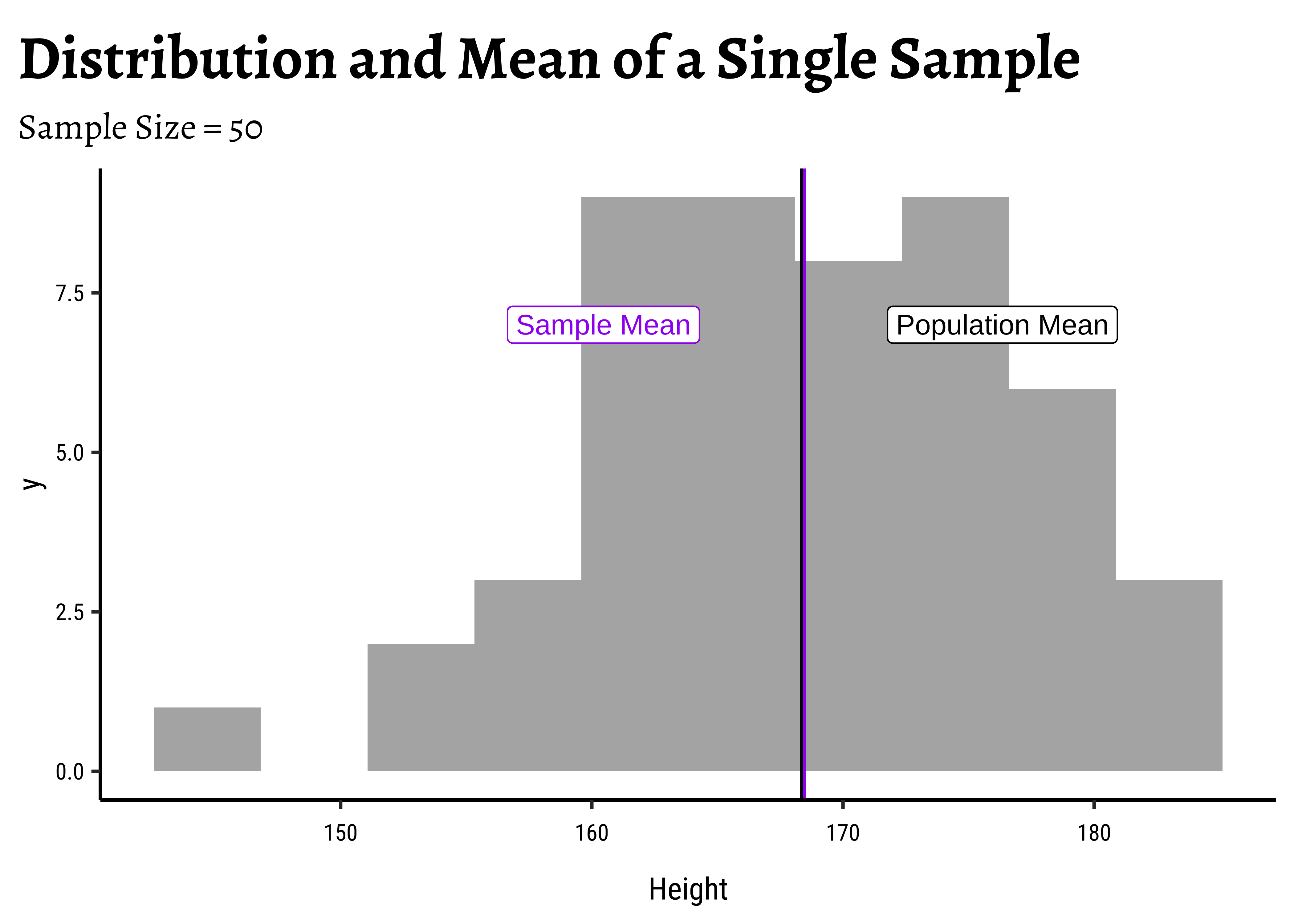
OK, so the sample_mean_50 is not too far from the pop_mean. Is this always true?

Let us check: we will create 500 repeated samples, each of size 50. And calculate their mean as the sample statistic, giving us a data frame containing 500 sample means. We will then see if these 500 means lie close to the pop_mean:

sample_50_500 <- do(500) * {
  sample(NHANES_adult, size = 50) %>%
    select(Height) %>% # drop sampling related column "orig.id"
    summarise(
      sample_mean = mean(Height),
      sample_sd = sd(Height),
      sample_min = min(Height),
      sample_max = max(Height)
    )
}
sample_50_500
dim(sample_50_500)

ABCDEFGHIJ0123456789

sample_mean <dbl>	sample_sd <dbl>	sample_min <dbl>	sample_max <dbl>	.row <int>	.index <dbl>
168.800	10.120841	149.7	192.6	1	1
169.068	10.001539	147.5	184.9	1	2
167.950	10.811507	146.4	186.8	1	3
167.184	9.243870	148.0	188.2	1	4
168.080	10.819502	144.4	186.8	1	5
169.926	8.830855	149.6	189.7	1	6
167.754	10.105590	143.9	186.3	1	7
167.970	10.807126	147.9	191.2	1	8
168.468	8.620229	152.7	186.3	1	9
168.550	11.802045	147.0	191.9	1	10

[1] 500   6

# Set graph theme
theme_set(new = theme_custom())
#

sample_50_500 %>%
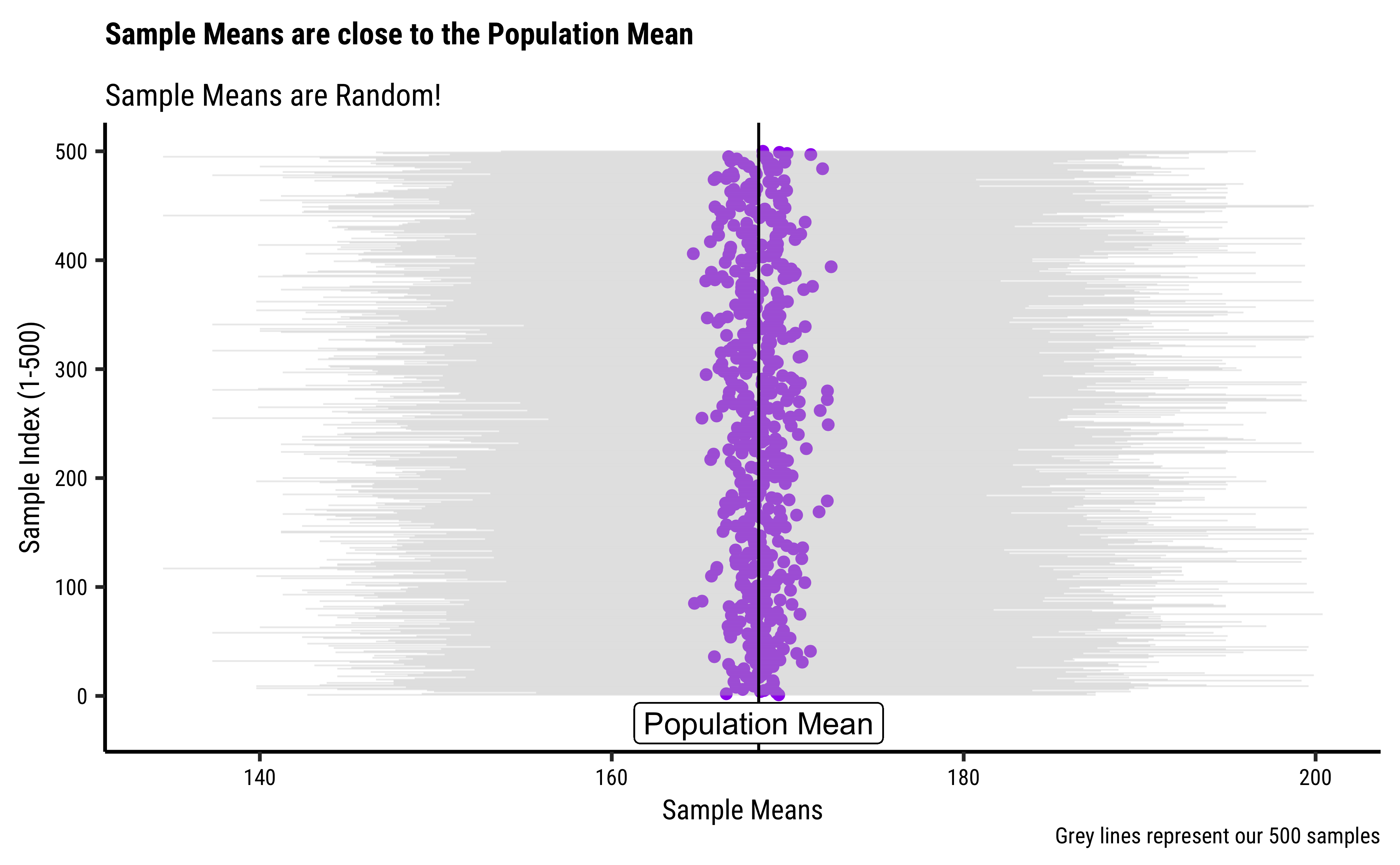
  gf_point(.index ~ sample_mean,
    color = "purple",
    title = "Sample Means are close to the Population Mean",
    subtitle = "Sample Means are Random!",
    caption = "Grey lines represent our 500 samples"
  ) %>%
  gf_segment(
    .index + .index ~ sample_min + sample_max,
    color = "grey",
    linewidth = 0.3,
    alpha = 0.3,
    ylab = "Sample Index (1-500)",
    xlab = "Sample Means"
  ) %>%
  gf_vline(
    xintercept = ~pop_mean,
    color = "black"
  ) %>%
  gf_label(-25 ~ pop_mean,
    label = "Population Mean",
    color = "black"
  )
##

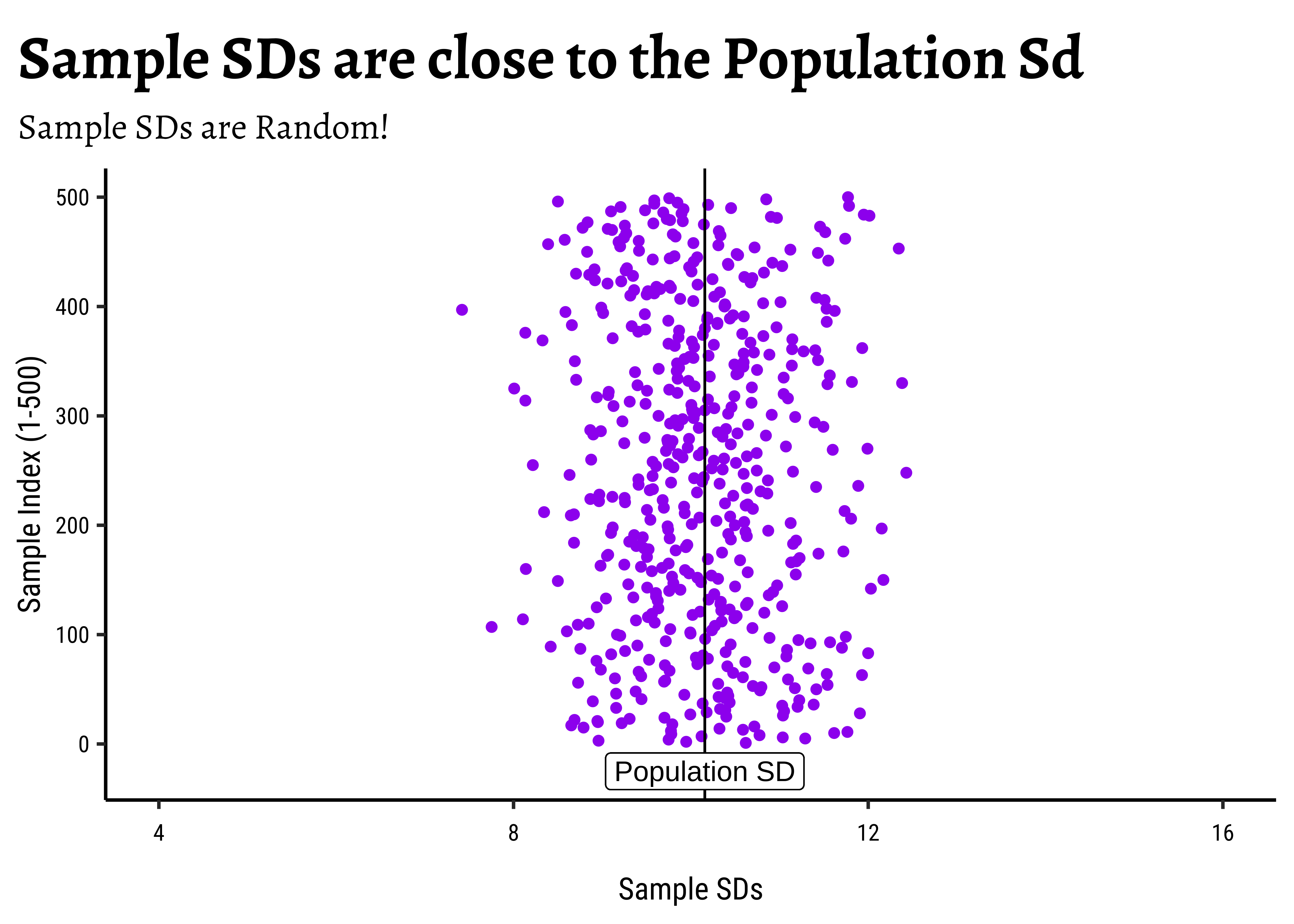
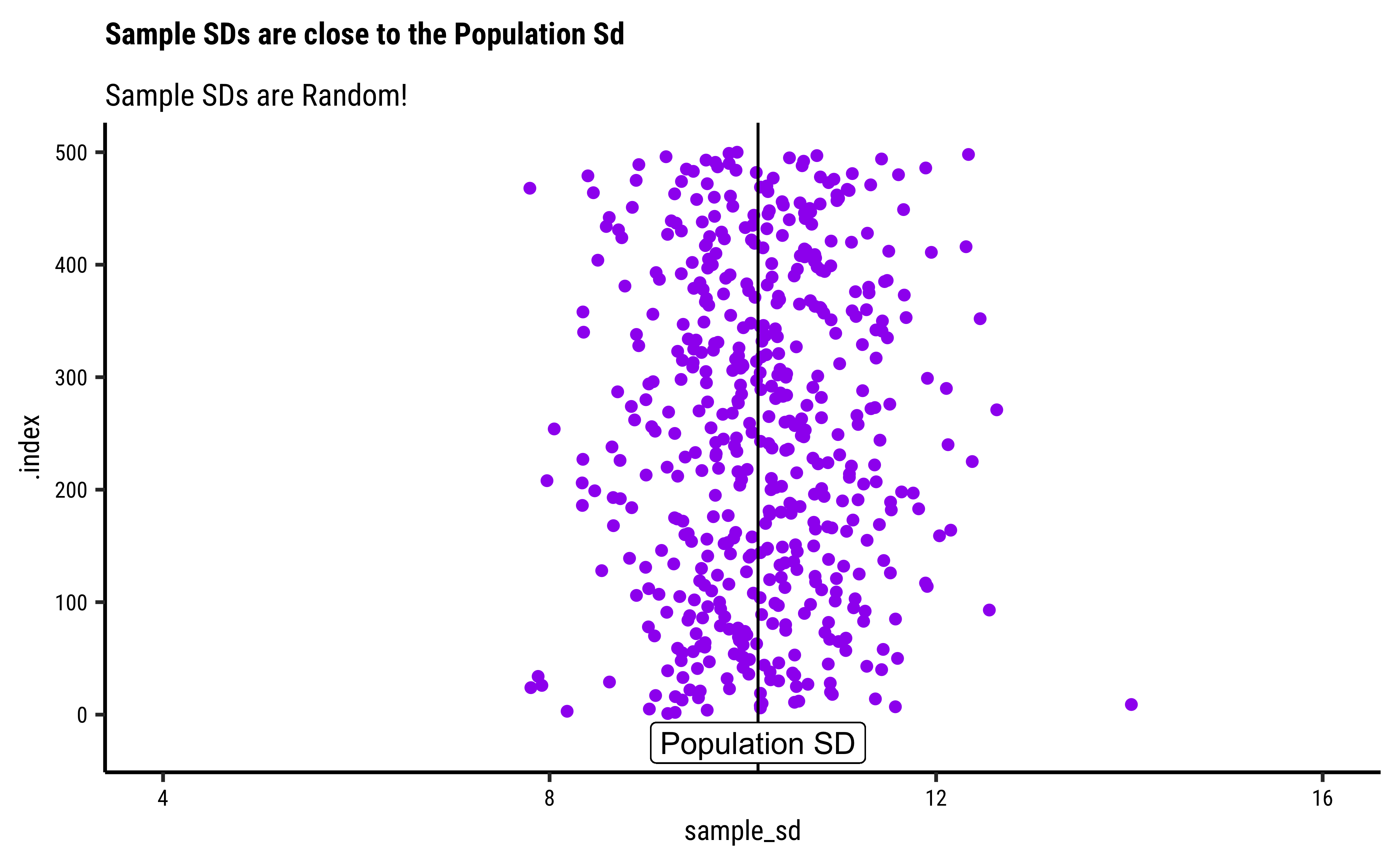
sample_50_500 %>%
  gf_point(.index ~ sample_sd,
    color = "purple",
    title = "Sample SDs are close to the Population Sd",
    subtitle = "Sample SDs are Random!",
  ) %>%
  gf_vline(
    xintercept = ~pop_sd,
    color = "black"
  ) %>%
  gf_label(-25 ~ pop_sd,
    label = "Population SD",
    color = "black"
  ) %>%
  gf_refine(lims(x = c(4, 16)))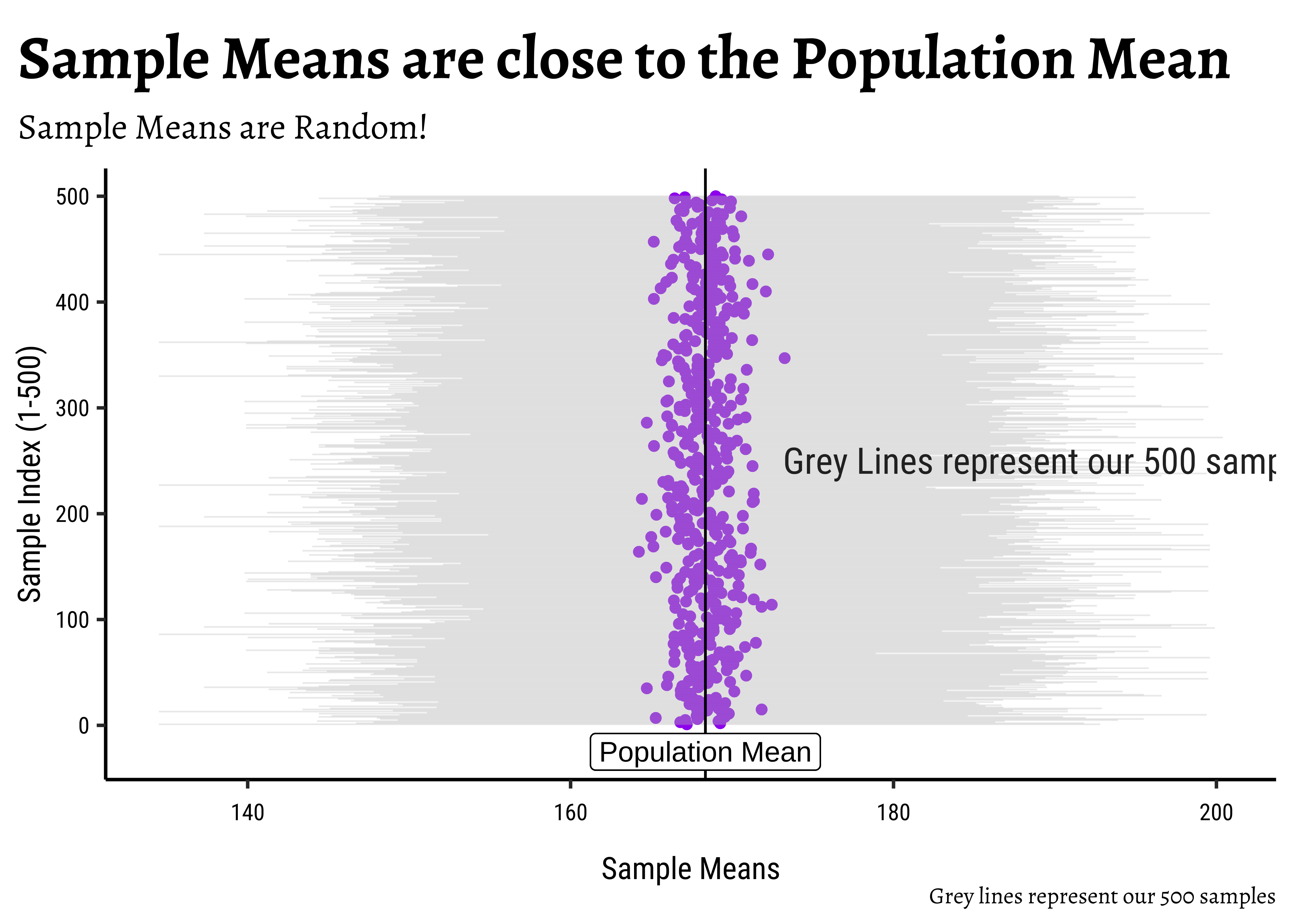

Sample Means and Sample SDs are a Random Variables!!¹

The sample_means (purple dots in the two graphs), are themselves random because the samples are random, of course. It appears that they are generally in the vicinity of the pop_mean (vertical black line). And hence they will have a mean and sd too 😱. Do not get confused ;-D

And the sample_sds are also random and have their own distribution, around the pop_sd.²

Distribution of Sample-Means

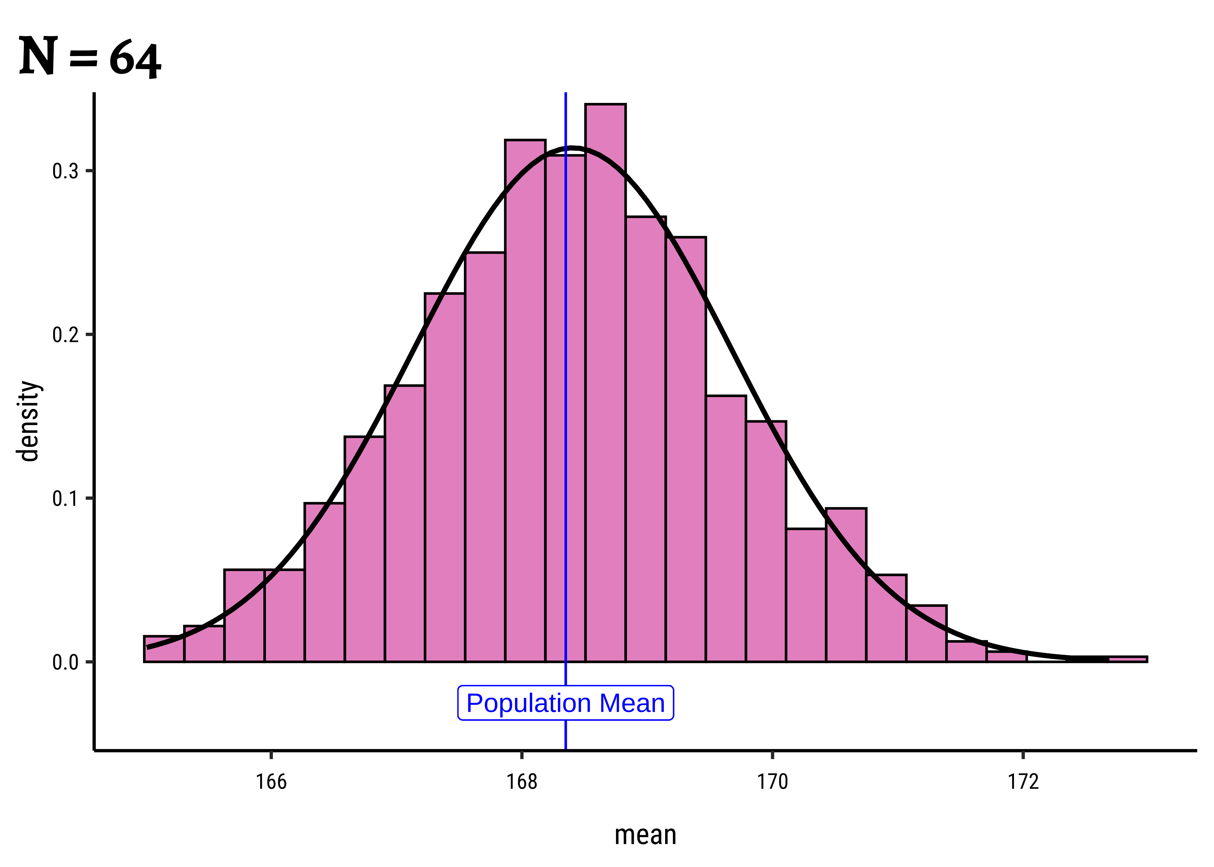
Since the sample-means are themselves random variables, let’s plot the distribution of these 500 sample-means themselves, called a distribution of sample-means. We will also plot the position of the population mean pop_mean parameter, the mean of the Height variable.

# Set graph theme
theme_set(new = theme_custom())
#

sample_50_500 %>%
  gf_dhistogram(~sample_mean, bins = 30, xlab = "Height") %>%
  gf_vline(
    xintercept = pop_mean,
    color = "blue"
  ) %>%
  gf_label(0.01 ~ pop_mean,
    label = "Population Mean",
    color = "blue"
  ) %>%
  gf_labs(
    title = "Sampling Mean Distribution",
    subtitle = "500 means"
  )


# How does this **distribution of sample-means** compare with the
# overall distribution of the population?
#
sample_50_500 %>%
  gf_dhistogram(~sample_mean, bins = 30, xlab = "Height") %>%
  gf_vline(
    xintercept = pop_mean,
    color = "blue"
  ) %>%
  gf_label(0.01 ~ pop_mean,
    label = "Population Mean",
    color = "blue"
  ) %>%
  ## Add the population histogram
  gf_histogram(~Height,
    data = NHANES_adult,
    alpha = 0.2, fill = "blue",
    bins = 30
  ) %>%
  gf_label(0.025 ~ (pop_mean + 20),
    label = "Population Distribution", color = "blue"
  ) %>%
  gf_labs(title = "Sampling Mean Distribution", subtitle = "Original Population overlay")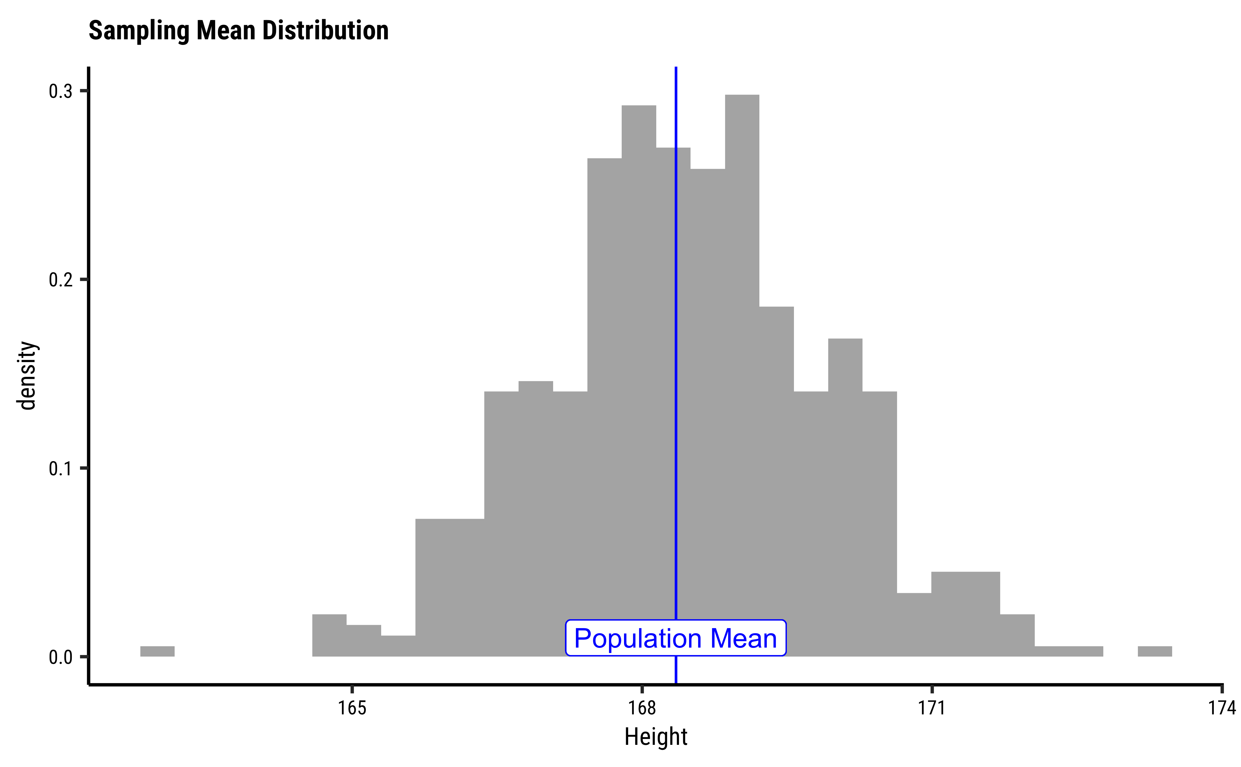

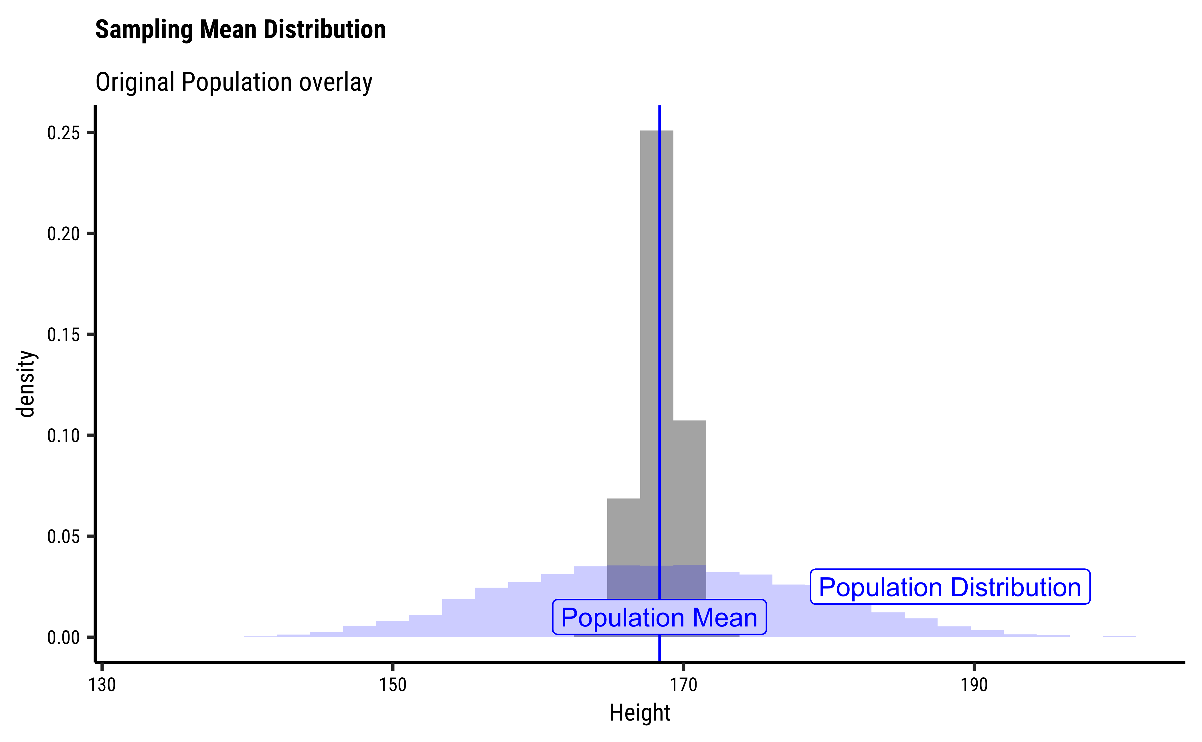
Distributions

Deriving the Central Limit Theorem (CLT)

We see in the Figure above that

the distribution of sample-means is centered around the pop_mean. ( Mean of the sample means = pop_mean!! 😱)
That the “spread” of the distribution of sample means is less than pop_sd. Curiouser and curiouser! But exactly how much is it?
And what is the kind of distribution?

One more experiment.

Now let’s repeatedly sample Height and compute the sample-means, and look at the resulting histograms. (We will deal with sample-standard-deviations shortly.) We will also use sample sizes of c(8, 16, ,32, 64) and generate 1000 samples each time, take the means and plot these 4 * 1000 means:

# set.seed(12345)

samples_08_1000 <- do(1000) * mean(resample(NHANES_adult$Height, size = 08))

samples_16_1000 <- do(1000) * mean(resample(NHANES_adult$Height, size = 16))

samples_32_1000 <- do(1000) * mean(resample(NHANES_adult$Height, size = 32))

samples_64_1000 <- do(1000) * mean(resample(NHANES_adult$Height, size = 64))

# samples_128_1000 <- do(1000) * mean(resample(NHANES_adult$Height, size = 128))

# Quick Check
head(samples_08_1000)

ABCDEFGHIJ0123456789

	mean <dbl>
1	165.3375
2	171.9125
3	169.2250
4	173.0875
5	164.8500
6	174.2250

Let us plot their individual histograms to compare them:

# Set graph theme
theme_set(new = theme_custom())
#
# Let us overlay their individual histograms to compare them:
p5 <- gf_dhistogram(~mean,
  data = samples_08_1000,
  color = "grey",
  fill = "dodgerblue", title = "N = 8"
) %>%
  gf_fitdistr(linewidth = 1) %>%
  gf_vline(
    xintercept = pop_mean, inherit = FALSE,
    color = "blue"
  ) %>%
  gf_label(-0.025 ~ pop_mean,
    label = "Population Mean",
    color = "blue"
  ) %>%
  gf_theme(scale_y_continuous(expand = expansion(mult = c(0.08, 0.02))))
##
p6 <- gf_dhistogram(~mean,
  data = samples_16_1000,
  color = "grey",
  fill = "sienna", title = "N = 16"
) %>%
  gf_fitdistr(linewidth = 1) %>%
  gf_vline(
    xintercept = pop_mean,
    color = "blue"
  ) %>%
  gf_label(-.025 ~ pop_mean,
    label = "Population Mean",
    color = "blue"
  ) %>%
  gf_theme(scale_y_continuous(expand = expansion(mult = c(0.08, 0.02))))
##
p7 <- gf_dhistogram(~mean,
  data = samples_32_1000,
  na.rm = TRUE,
  color = "grey",
  fill = "palegreen", title = "N = 32"
) %>%
  gf_fitdistr(linewidth = 1) %>%
  gf_vline(
    xintercept = pop_mean,
    color = "blue"
  ) %>%
  gf_label(-.025 ~ pop_mean,
    label = "Population Mean", color = "blue"
  ) %>%
  gf_theme(scale_y_continuous(expand = expansion(mult = c(0.08, 0.02))))

p8 <- gf_dhistogram(~mean,
  data = samples_64_1000,
  na.rm = TRUE,
  color = "grey",
  fill = "violetred", title = "N = 64"
) %>%
  gf_fitdistr(linewidth = 1) %>%
  gf_vline(
    xintercept = pop_mean,
    color = "blue"
  ) %>%
  gf_label(-.025 ~ pop_mean,
    label = "Population Mean", color = "blue"
  ) %>%
  gf_theme(scale_y_continuous(expand = expansion(mult = c(0.08, 0.02))))

# patchwork::wrap_plots(p5,p6,p7,p8)
p5
p6
p7
p8

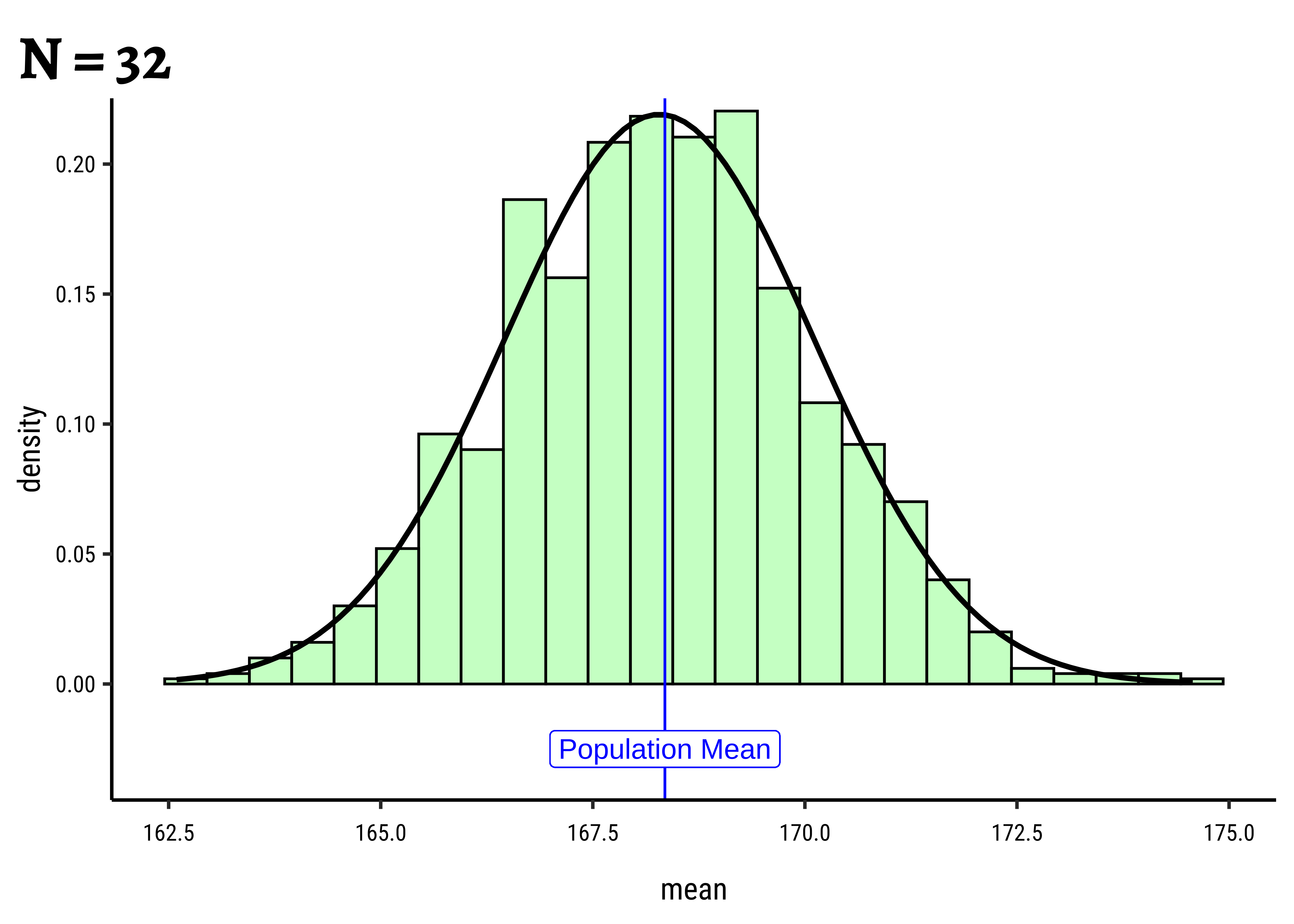
And if we overlay these histograms on top of one another:

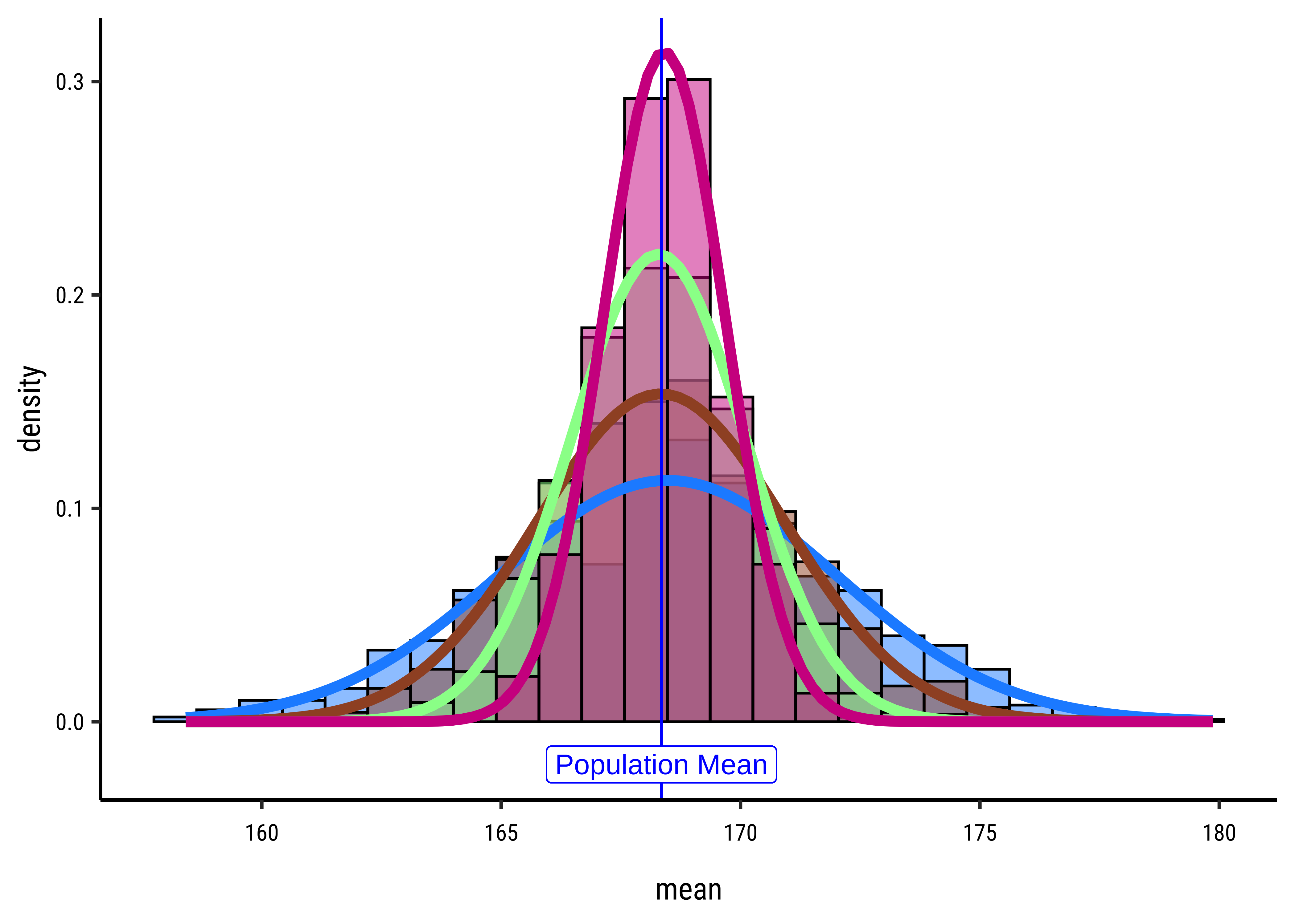
From the histograms we learn that the sample-means are normally distributed around the population mean. This feels intuitively right because when we sample from the population, many values will be close to the population mean, and values far away from the mean will be increasingly scarce.

Let us calculate the means of the sample-distributions:

mean(~mean, data = samples_08_1000) # Mean of means!!!;-0
mean(~mean, data = samples_16_1000)
mean(~mean, data = samples_32_1000)
mean(~mean, data = samples_64_1000)
pop_mean

[1] 168.1511

[1] 168.353

[1] 168.3914

[1] 168.3819

[1] 168.3497

All are pretty close to the population mean !!!

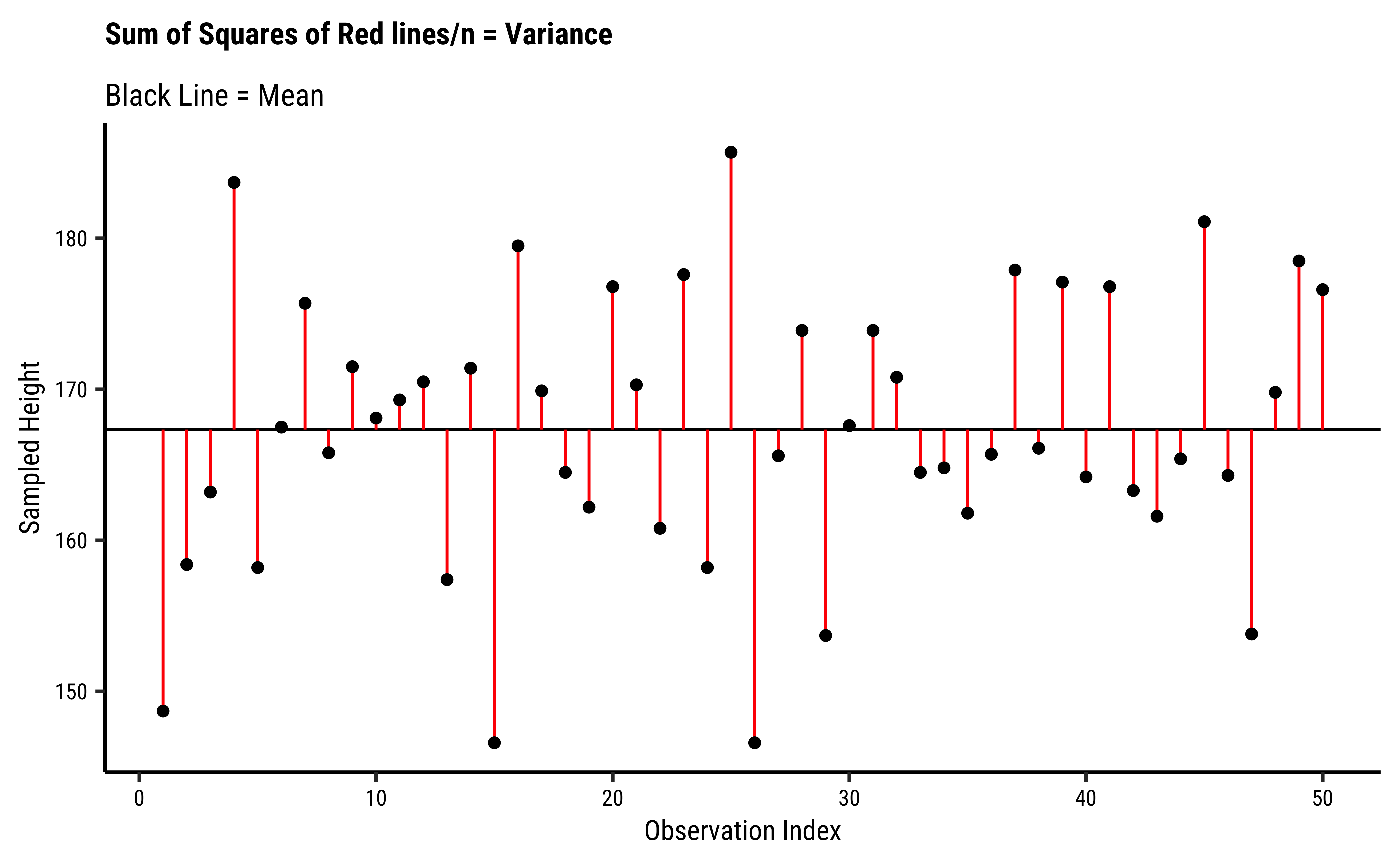
Consider the standard deviations of the sampling distributions:

$s d_{i} = \sqrt{\frac{Σ [x_{i} - \bar{x_{i}}]^{2}}{n_{i}}}$

We take the sum of all squared differences from the mean in a sample. If we divide this sum-of-squared-differences by the sample length $n$ , we get a sort of average squared difference, or per-capita squared error from the mean, which is called the variance.

Taking the square root gives us an average error, which we would call, of course, the standard deviation.

pop_sd
sd(~mean, data = samples_08_1000)
sd(~mean, data = samples_16_1000)
sd(~mean, data = samples_32_1000)
sd(~mean, data = samples_64_1000)

[1] 10.15705

[1] 3.682819

[1] 2.5176

[1] 1.775868

[1] 1.25669

These are also decreasing steadily with sample size. How are they related to the pop_sd?

pop_sd
pop_sd / sqrt(8)
pop_sd / sqrt(16)
pop_sd / sqrt(32)
pop_sd / sqrt(64)

[1] 10.15705

[1] 3.591058

[1] 2.539262

[1] 1.795529

[1] 1.269631

As we can see, the standard deviations of the sampling-mean-distributions is inversely proportional to the squre root of lengths of the sample.

Central Limit Theorem

Now we have enough to state the Central Limit Theorem (CLT)

the sample-means are normally distributed around the population mean. So any mean of a single sample is a good, unbiased estimate for the pop_mean
the sample-mean distributions narrow with sample length, i.e their sd decreases with increasing sample size.
$s d \sim \frac{1}{s q r t (n)}$
This is regardless of the distribution of the population itself.³

This theorem underlies all our procedures and techniques for statistical inference, as we shall see.

The Standard Error

Consider once again the standard deviations in each of the sample-distributions that we have generated. As we saw these decrease with sample size.

sd = pop_sd/sqrt(sample_size)where sample-size⁴ here is one of c(8, 16, 32, 64).

We reserve the term Standard Deviation for the population, and name this computed standard deviation of the sample-mean-distributions as the Standard Error. This statistic derived from the sample-mean-distribution will help us infer our population parameters with a precise estimate of the uncertainty involved.

$S t a n d a r d E r r o r s e s e = \frac{p o p . s d}{\sqrt{n}}$ However, we don’t normally know the pop_sd!! So now what?? So is this chicken and egg??

Let us take SINGLE SAMPLES of each size, as we normally would:

sample_08 <- mosaic::sample(NHANES_adult, size = 8) %>%
  select(Height)
sample_16 <- mosaic::sample(NHANES_adult, size = 16) %>%
  select(Height)
sample_32 <- mosaic::sample(NHANES_adult, size = 32) %>%
  select(Height)
sample_64 <- mosaic::sample(NHANES_adult, size = 64) %>%
  select(Height)
##
sd(~Height, data = sample_08)

[1] 7.427555

sd(~Height, data = sample_16)

[1] 7.710034

sd(~Height, data = sample_32)

[1] 8.803592

sd(~Height, data = sample_64)

[1] 10.10828

Warning

As we saw at the start of this module, the sample-means are distributed around the pop_mean, AND it appears that the sample-sds are also distributed around the pop_sd!

However, the sample-sd distribution is not Gaussian, and the sample_sd is also not an unbiased estimate for the pop_sd. However, when the sample size $n$ is large ( $n >= 30$ ), the sample-sd distribution approximates the Gaussian, and the bias is small.

And so, in the same way, we approximate the pop_sd with the sd of a single sample of the same length. Hence the Standard Error can be computed from a single sample as:

$S t a n d a r d E r r o r s e s e = \frac{s a m p l e . s d}{\sqrt{n}}$

With these, the Standard Errors(SE) evaluate to:

pop_sd <- sd(~Height, data = NHANES_adult)
pop_sd
sd(~Height, data = sample_08) / sqrt(8)
sd(~Height, data = sample_16) / sqrt(16)
sd(~Height, data = sample_32) / sqrt(32)
sd(~Height, data = sample_64) / sqrt(64)

[1] 10.15705

[1] 2.626037

[1] 1.927509

[1] 1.55627

[1] 1.263536

Confidence intervals

When we work with samples, we want to be able to speak with a certain degree of confidence about the population mean, based on the evaluation of one sample mean, not a large number of them. Given that sample-means are normally distributed around the pop_mean, we can say that $68 %$ of all possible sample-mean lie within $\pm S E$ of the population mean; and further that $95 %$ of all possible sample-mean lie within $\pm 2 * S E$ of the population mean. These two constants $\pm 1$ and $\pm 2$ are the z-scores from the z-distribution we saw earlier:

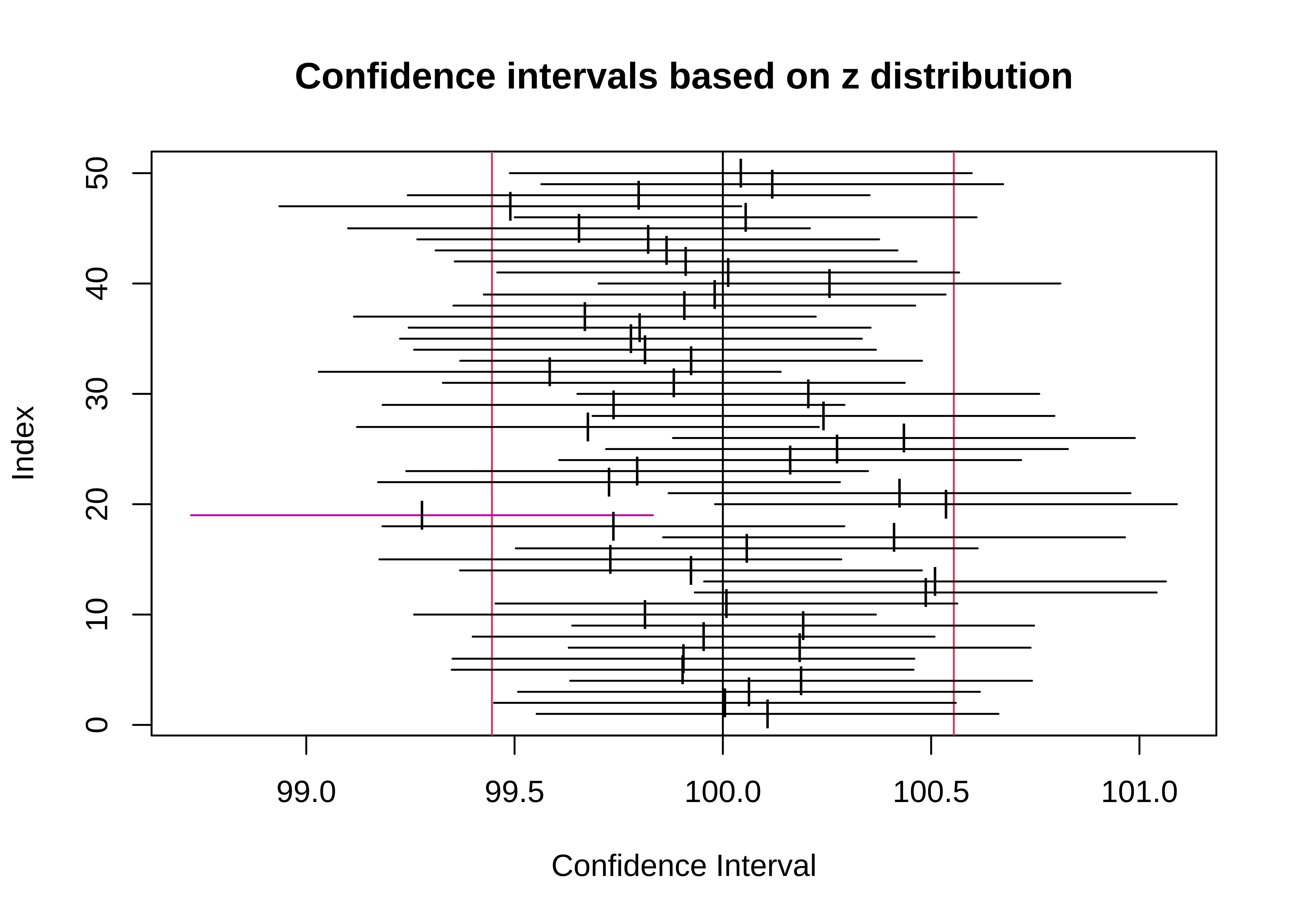
These two intervals $s a m p l e . m e a n \pm S E$ and $s a m p l e . m e a n \pm 2 * S E$ are called the confidence intervals for the population mean, at levels $68 %$ and $95 %$ probability respectively.

How do these vary with sample size $n$ ?f

# Set graph theme
theme_set(new = theme_custom())
#
tbl_1 <- get_ci(samples_08_1000, level = 0.95)
tbl_2 <- get_ci(samples_16_1000, level = 0.95)
tbl_3 <- get_ci(samples_32_1000, level = 0.95)
tbl_4 <- get_ci(samples_64_1000, level = 0.95)
rbind(tbl_1, tbl_2, tbl_3, tbl_4) %>%
  rownames_to_column("index") %>%
  cbind("sample_size" = c(8, 16, 32, 64)) %>%
  gf_segment(index + index ~ lower_ci + upper_ci) %>%
  gf_vline(xintercept = pop_mean) %>%
  gf_labs(
    title = "95% Confidence Intervals for the Mean",
    subtitle = "Varying samples sizes 8-16-32-64",
    y = "Sample Size", x = "Mean Ranges"
  ) %>%
  gf_refine(scale_y_discrete(labels = c(8, 16, 32, 64))) %>%
  gf_refine(annotate(geom = "label", x = pop_mean + 1.75, y = 1.5, label = "Population Mean"))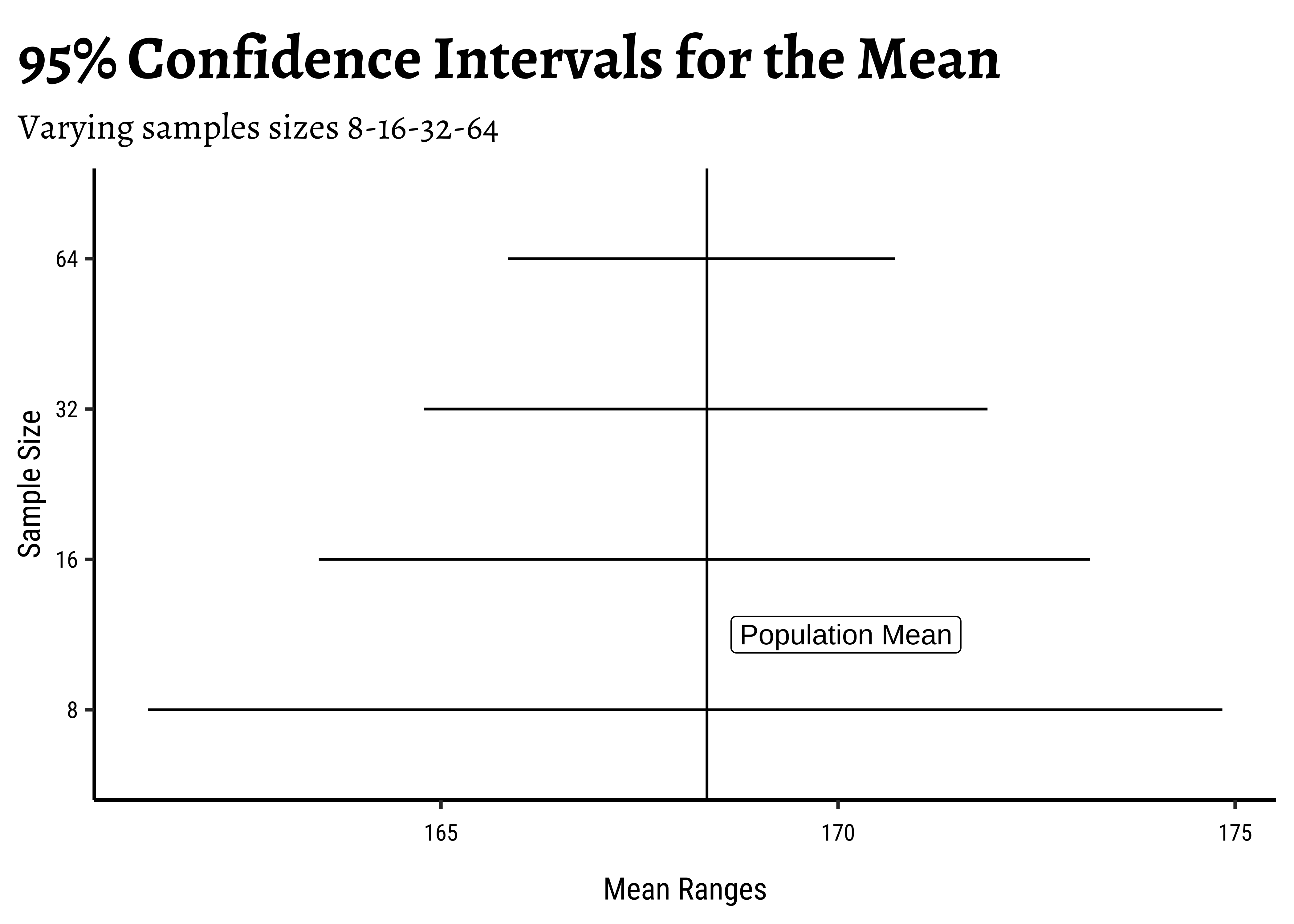

Confidence Intervals Shrink!

Yes, with sample size! Why is that a good thing?

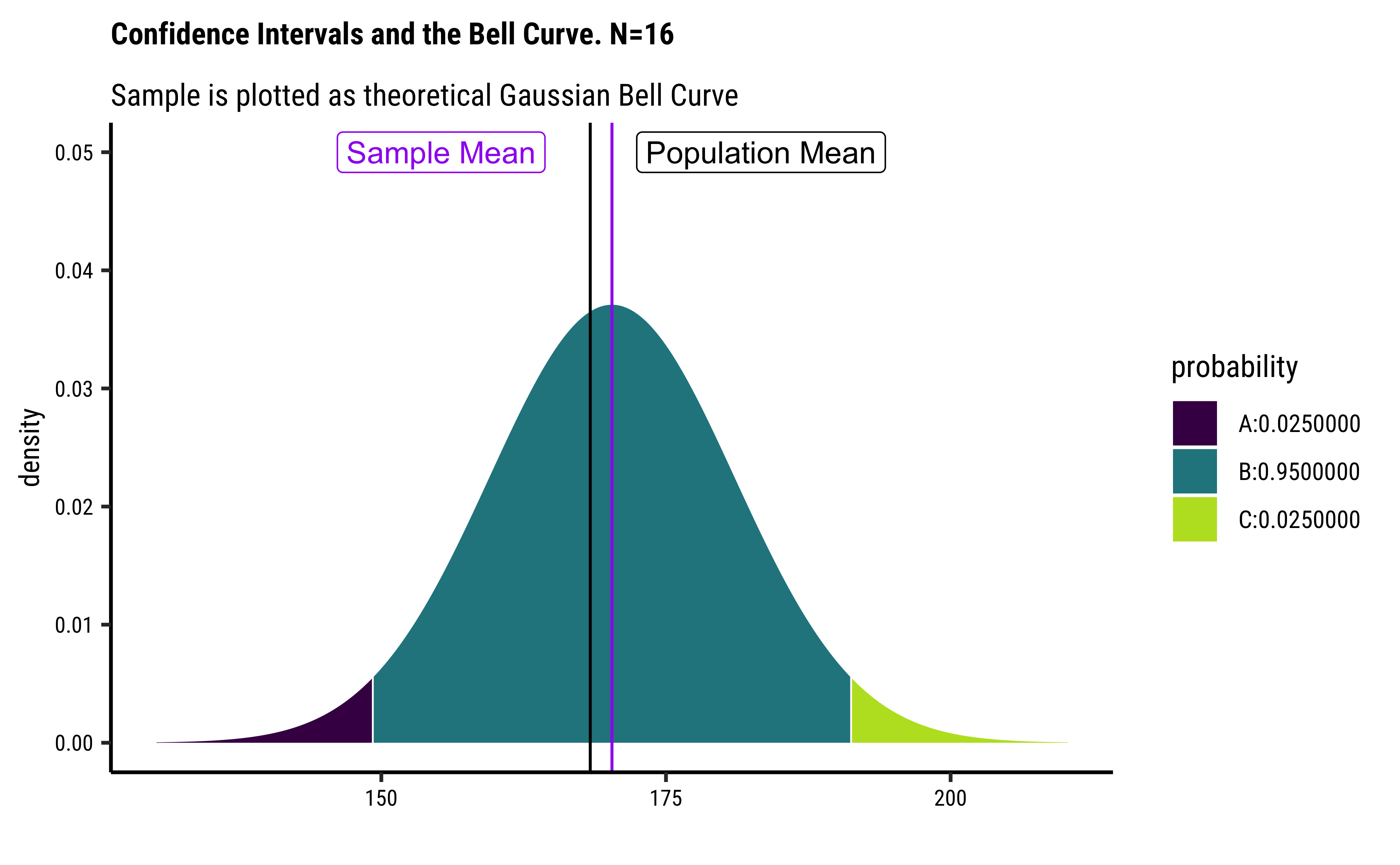
So finally, we can pretend that our sample is also distributed normally ( i.e Gaussian) and use its sample_sd as a substitute for pop_sd, plot the standard errors on the sample histogram, and see where our believed mean is.

# Set graph theme
theme_set(new = theme_custom())
#
sample_mean <- mean(~Height, data = sample_16)
se <- sd(~Height, data = sample_16) / sqrt(16)
#
xqnorm(
  p = c(0.025, 0.975),
  mean = sample_mean,
  sd = sd(~Height, data = sample_16),
  return = c("plot"), verbose = F
) %>%
  gf_vline(xintercept = ~pop_mean, colour = "black") %>%
  gf_vline(xintercept = mean(~Height, data = sample_16), colour = "purple") %>%
  gf_labs(
    title = "Confidence Intervals and the Bell Curve. N=16",
    subtitle = "Sample is plotted as theoretical Gaussian Bell Curve"
  ) %>%
  gf_refine(
    annotate(geom = "label", x = pop_mean + 15, y = 0.05, label = "Population Mean"),
    annotate(geom = "label", x = sample_mean - 15, y = 0.05, label = "Sample Mean", colour = "purple")
  )

pop_mean
se <- sd(~Height, data = sample_16) / sqrt(16)
mean(~Height, data = sample_16) - 2.0 * se
mean(~Height, data = sample_16) + 2.0 * se

[1] 168.3497
[1] 166.2512
[1] 173.9613

So if our believed mean is within the Confidence Intervals, then OK, we can say our belief may be true. If it is way outside the confidence intervals, we have to think that our belief may be flawed and accept and alternative interpretation.

CLT Workflow

Thus if we want to estimate a population mean:

we take one random sample from the population of length $n$
we calculate the mean from the sample sample-mean
we calculate the sample-sd
we calculate the Standard Error as $\frac{s a m p l e - s d}{\sqrt{n}}$
we calculate 95% confidence intervals for the population parameter based on the formula $C I_{95 %} = s a m p l e . m e a n \pm 2 * S E$ .
Since Standard Error decreases with sample size, we need to make our sample of adequate size.( $n = 30$ seems appropriate in most cases. Why?)
And we do not have to worry about the distribution of the population. It need not be normal/Gaussian/Bell-shaped !!

CLT Assumptions

Sample is of “decent length” $n >= 30$ ;
Therefore sample histogram is Gaussian

An interactive Sampling app

Here below is an interactive sampling app. Play with the different settings, especially the distribution in the population to get a firm grasp on Sampling and the CLT.

https://gallery.shinyapps.io/CLT_mean/

References

Diez, David M & Barr, Christopher D & Çetinkaya-Rundel, Mine, OpenIntro Statistics. https://www.openintro.org/book/os/
Stats Test Wizard. https://www.socscistatistics.com/tests/what_stats_test_wizard.aspx
Diez, David M & Barr, Christopher D & Çetinkaya-Rundel, Mine: OpenIntro Statistics. Available online https://www.openintro.org/book/os/
Måns Thulin, Modern Statistics with R: From wrangling and exploring data to inference and predictive modelling http://www.modernstatisticswithr.com/
Jonas Kristoffer Lindeløv, Common statistical tests are linear models (or: how to teach stats) https://lindeloev.github.io/tests-as-linear/
CheatSheet https://lindeloev.github.io/tests-as-linear/linear_tests_cheat_sheet.pdf
Common statistical tests are linear models: a work through by Steve Doogue https://steverxd.github.io/Stat_tests/
Jeffrey Walker “Elements of Statistical Modeling for Experimental Biology”. https://www.middleprofessor.com/files/applied-biostatistics_bookdown/_book/
Adam Loy, Lendie Follett & Heike Hofmann (2016) Variations of Q–Q Plots: The Power of Our Eyes!, The American Statistician, 70:2, 202-214, DOI: 10.1080/00031305.2015.1077728

R Package Citations

Package	Version	Citation
NHANES	2.1.0	Pruim (2015)
regressinator	0.2.0	Reinhart (2024)
smovie	1.1.6	Northrop (2023)
TeachHist	0.2.1	Lange (2023)
TeachingDemos	2.13	Snow (2024)
visualize	4.5.0	Balamuta (2023)

Balamuta, James. 2023. visualize: Graph Probability Distributions with User Supplied Parameters and Statistics. https://CRAN.R-project.org/package=visualize.

Lange, Carsten. 2023. TeachHist: A Collection of Amended Histograms Designed for Teaching Statistics. https://CRAN.R-project.org/package=TeachHist.

Northrop, Paul J. 2023. smovie: Some Movies to Illustrate Concepts in Statistics. https://CRAN.R-project.org/package=smovie.

Pruim, Randall. 2015. NHANES: Data from the US National Health and Nutrition Examination Study. https://CRAN.R-project.org/package=NHANES.

Reinhart, Alex. 2024. regressinator: Simulate and Diagnose (Generalized) Linear Models. https://CRAN.R-project.org/package=regressinator.

Snow, Greg. 2024. TeachingDemos: Demonstrations for Teaching and Learning. https://CRAN.R-project.org/package=TeachingDemos.

Footnotes

https://stats.libretexts.org/Bookshelves/Introductory_Statistics/Introductory_Statistics_(Shafer_and_Zhang)/06%3A_Sampling_Distributions/6.01%3A_The_Mean_and_Standard_Deviation_of_the_Sample_Mean ↩︎
https://mathworld.wolfram.com/StandardDeviationDistribution.html ↩︎
The `Height` variable seems to be normally distributed at population level. We will try other non-normal population variables as an exercise in the tutorials.↩︎
Once sample size = population, we have complete access to the population and there is no question of estimation error! So sample_sd = pop_sd!↩︎

Citation

BibTeX citation:

@online{2022,
  author = {},
  title = {🎲 {Samples,} {Populations,} {Statistics} and {Inference}},
  date = {2022-11-25},
  url = {https://av-quarto.netlify.app/content/courses/Analytics/Inference/Modules/20-SampProb/},
  langid = {en},
  abstract = {How much \textasciitilde\textasciitilde
    Land\textasciitilde\textasciitilde{} Data does a Man need?}
}

For attribution, please cite this work as:

“🎲 Samples, Populations, Statistics and Inference.” 2022. November 25, 2022. https://av-quarto.netlify.app/content/courses/Analytics/Inference/Modules/20-SampProb/.