Random Forests

Author

Arvind V.

Published

January 6, 2021

Modified

July 29, 2025

knitr::opts_chunk$set(echo = TRUE)
library(tidyverse)
library(broom)
library(prettydoc)
library(corrplot)
library(ggformula)
library(palmerpenguins) # Allison Horst's `penguins` data.
##
library(tidymodels)
library(dials)
library(modeldata)
library(rsample)
library(recipes)
library(yardstick)
library(parsnip)

Penguin Random Forest Model with`randomForest`

Using the penguins dataset and Random Forest Classification.

penguins

ABCDEFGHIJ0123456789

species <fct>	island <fct>	bill_length_mm <dbl>	bill_depth_mm <dbl>	flipper_length_mm <int>	body_mass_g <int>	sex <fct>	year <int>
Adelie	Torgersen	39.1	18.7	181	3750	male	2007
Adelie	Torgersen	39.5	17.4	186	3800	female	2007
Adelie	Torgersen	40.3	18.0	195	3250	female	2007
Adelie	Torgersen	NA	NA	NA	NA	NA	2007
Adelie	Torgersen	36.7	19.3	193	3450	female	2007
Adelie	Torgersen	39.3	20.6	190	3650	male	2007
Adelie	Torgersen	38.9	17.8	181	3625	female	2007
Adelie	Torgersen	39.2	19.6	195	4675	male	2007
Adelie	Torgersen	34.1	18.1	193	3475	NA	2007
Adelie	Torgersen	42.0	20.2	190	4250	NA	2007

summary(penguins)

      species          island    bill_length_mm  bill_depth_mm  
 Adelie   :152   Biscoe   :168   Min.   :32.10   Min.   :13.10  
 Chinstrap: 68   Dream    :124   1st Qu.:39.23   1st Qu.:15.60  
 Gentoo   :124   Torgersen: 52   Median :44.45   Median :17.30  
                                 Mean   :43.92   Mean   :17.15  
                                 3rd Qu.:48.50   3rd Qu.:18.70  
                                 Max.   :59.60   Max.   :21.50  
                                 NA's   :2       NA's   :2      
 flipper_length_mm  body_mass_g       sex           year     
 Min.   :172.0     Min.   :2700   female:165   Min.   :2007  
 1st Qu.:190.0     1st Qu.:3550   male  :168   1st Qu.:2007  
 Median :197.0     Median :4050   NA's  : 11   Median :2008  
 Mean   :200.9     Mean   :4202                Mean   :2008  
 3rd Qu.:213.0     3rd Qu.:4750                3rd Qu.:2009  
 Max.   :231.0     Max.   :6300                Max.   :2009  
 NA's   :2         NA's   :2

penguins %>% skimr::skim()

Data summary
Name	Piped data
Number of rows	344
Number of columns	8
_______________________
Column type frequency:
factor	3
numeric	5
________________________
Group variables	None

Variable type: factor

skim_variable	n_missing	complete_rate	ordered	n_unique	top_counts
species	0	1.00	FALSE	3	Ade: 152, Gen: 124, Chi: 68
island	0	1.00	FALSE	3	Bis: 168, Dre: 124, Tor: 52
sex	11	0.97	FALSE	2	mal: 168, fem: 165

Variable type: numeric

skim_variable	n_missing	complete_rate	mean	sd	p0	p25	p50	p75	p100	hist
bill_length_mm	2	0.99	43.92	5.46	32.1	39.23	44.45	48.5	59.6	▃▇▇▆▁
bill_depth_mm	2	0.99	17.15	1.97	13.1	15.60	17.30	18.7	21.5	▅▅▇▇▂
flipper_length_mm	2	0.99	200.92	14.06	172.0	190.00	197.00	213.0	231.0	▂▇▃▅▂
body_mass_g	2	0.99	4201.75	801.95	2700.0	3550.00	4050.00	4750.0	6300.0	▃▇▆▃▂
year	0	1.00	2008.03	0.82	2007.0	2007.00	2008.00	2009.0	2009.0	▇▁▇▁▇

penguins <- penguins %>% tidyr::drop_na()
# Spent one hour trying to find `drop-na()` (14 June 2020)

# library(corrplot)
cor <- penguins %>%
  select(where(is.numeric)) %>%
  cor()
cor %>% corrplot(., method = "ellipse", order = "hclust", tl.cex = 1.0, )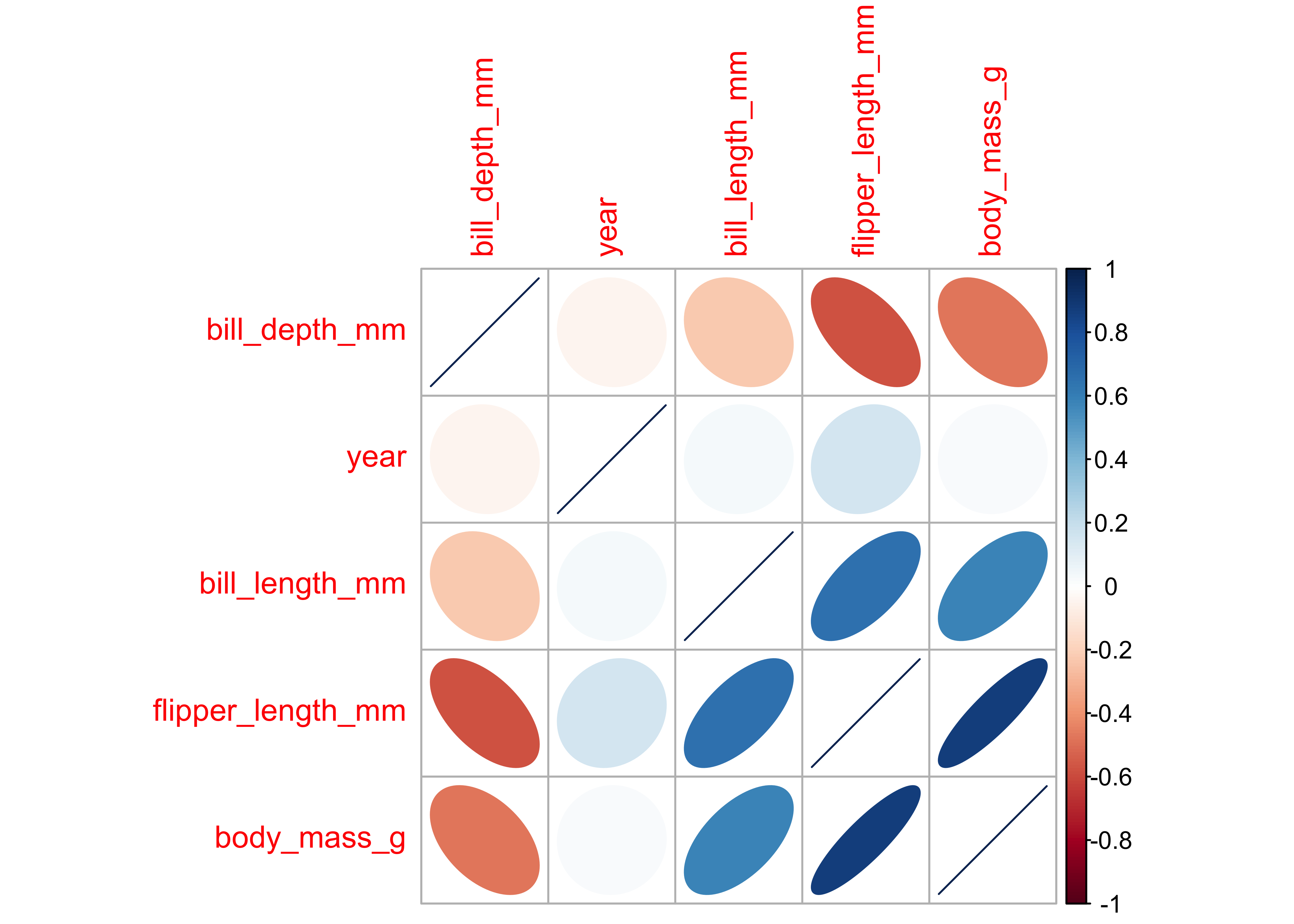

# try these too:
# cor %>% corrplot(., method = "square", order = "hclust",tl.cex = 0.5)
# cor %>% corrplot(., method = "color", order = "hclust",tl.cex = 0.5)
# cor %>% corrplot(., method = "shade", order = "hclust",tl.cex = 0.5)

Notes: - flipper_length_mm and culmen_depth_mm are negatively correlated at approx (-0.7) - flipper_length_mm and body_mass_g are positively correlated at approx 0.8

So we will use steps in the recipe to remove correlated variables.

Penguin Data Sampling and Recipe

# Data Split
penguin_split <- initial_split(penguins, prop = 0.6)
penguin_train <- training(penguin_split)
penguin_test <- testing(penguin_split)
penguin_split

<Training/Testing/Total>
<199/134/333>

head(penguin_train)

ABCDEFGHIJ0123456789

species <fct>	island <fct>	bill_length_mm <dbl>	bill_depth_mm <dbl>	flipper_length_mm <int>	body_mass_g <int>	sex <fct>	year <int>
Gentoo	Biscoe	47.5	14.0	212	4875	female	2009
Gentoo	Biscoe	46.2	14.5	209	4800	female	2007
Adelie	Dream	36.0	17.8	195	3450	female	2009
Chinstrap	Dream	46.4	18.6	190	3450	female	2007
Gentoo	Biscoe	42.6	13.7	213	4950	female	2008
Gentoo	Biscoe	45.1	14.5	215	5000	female	2007

# Recipe
penguin_recipe <- penguins %>%
  recipe(species ~ .) %>%
  step_normalize(all_numeric()) %>% # Scaling and Centering
  step_corr(all_numeric()) %>% # Handling correlated variables
  prep()

# Baking the data
penguin_train_baked <- penguin_train %>%
  bake(object = penguin_recipe, new_data = .)

penguin_test_baked <- penguin_test %>%
  bake(object = penguin_recipe, new_data = .)

head(penguin_train_baked)

ABCDEFGHIJ0123456789

island <fct>	bill_length_mm <dbl>	bill_depth_mm <dbl>	flipper_length_mm <dbl>	body_mass_g <dbl>	sex <fct>	year <dbl>	species <fct>
Biscoe	0.6413275	-1.6071541	0.7871873	0.8295204	female	1.1783814	Gentoo
Biscoe	0.4036096	-1.3532485	0.5731427	0.7363777	female	-1.2818130	Gentoo
Dream	-1.4615611	0.3225288	-0.4257325	-0.9401915	female	1.1783814	Adelie
Dream	0.4401816	0.7287778	-0.7824736	-0.9401915	female	-1.2818130	Chinstrap
Biscoe	-0.2546859	-1.7594975	0.8585356	0.9226631	female	-0.0517158	Gentoo
Biscoe	0.2024638	-1.3532485	1.0012320	0.9847583	female	-1.2818130	Gentoo

Penguin Random Forest Model

penguin_model <-
  rand_forest(trees = 100) %>%
  set_engine("randomForest") %>%
  set_mode("classification")
penguin_model

Random Forest Model Specification (classification)

Main Arguments:
  trees = 100

Computational engine: randomForest

penguin_fit <-
  penguin_model %>%
  fit(species ~ ., penguin_train_baked)
penguin_fit

parsnip model object


Call:
 randomForest(x = maybe_data_frame(x), y = y, ntree = ~100) 
               Type of random forest: classification
                     Number of trees: 100
No. of variables tried at each split: 2

        OOB estimate of  error rate: 2.01%
Confusion matrix:
          Adelie Chinstrap Gentoo class.error
Adelie        86         2      0  0.02272727
Chinstrap      2        38      0  0.05000000
Gentoo         0         0     71  0.00000000

# iris_ranger <-
#   rand_forest(trees = 100) %>%
#   set_mode("classification") %>%
#   set_engine("ranger") %>%
#   fit(Species ~ ., data = iris_training_baked)

Metrics for the Penguin Random Forest Model

# Predictions
predict(object = penguin_fit, new_data = penguin_test_baked) %>%
  dplyr::bind_cols(penguin_test_baked) %>%
  glimpse()

Rows: 134
Columns: 9
$ .pred_class       <fct> Adelie, Adelie, Adelie, Adelie, Adelie, Adelie, Adel…
$ island            <fct> Torgersen, Torgersen, Torgersen, Biscoe, Biscoe, Bis…
$ bill_length_mm    <dbl> -1.3335592, -1.7541369, 0.3670377, -1.0592694, -0.62…
$ bill_depth_mm     <dbl> 1.08424573, 0.62721557, 2.20143056, 0.47487218, 0.72…
$ flipper_length_mm <dbl> -0.56842897, -1.21056301, -0.49708074, -1.13921478, …
$ body_mass_g       <dbl> -0.940191505, -1.095429393, -0.008764181, -0.3192399…
$ sex               <fct> female, female, male, male, male, male, female, fema…
$ year              <dbl> -1.2818130, -1.2818130, -1.2818130, -1.2818130, -1.2…
$ species           <fct> Adelie, Adelie, Adelie, Adelie, Adelie, Adelie, Adel…

# Prediction Accuracy Metrics
predict(object = penguin_fit, new_data = penguin_test_baked) %>%
  dplyr::bind_cols(penguin_test_baked) %>%
  yardstick::metrics(truth = species, estimate = .pred_class)

ABCDEFGHIJ0123456789

.metric <chr>	.estimator <chr>	.estimate <dbl>
accuracy	multiclass	0.9701493
kap	multiclass	0.9531632

# Prediction Probabilities
penguin_fit_probs <-
  predict(penguin_fit, penguin_test_baked, type = "prob") %>%
  dplyr::bind_cols(penguin_test_baked)
glimpse(penguin_fit_probs)

Rows: 134
Columns: 11
$ .pred_Adelie      <dbl> 0.99, 0.99, 0.59, 1.00, 1.00, 1.00, 0.84, 0.95, 0.92…
$ .pred_Chinstrap   <dbl> 0.01, 0.01, 0.39, 0.00, 0.00, 0.00, 0.16, 0.05, 0.08…
$ .pred_Gentoo      <dbl> 0.00, 0.00, 0.02, 0.00, 0.00, 0.00, 0.00, 0.00, 0.00…
$ island            <fct> Torgersen, Torgersen, Torgersen, Biscoe, Biscoe, Bis…
$ bill_length_mm    <dbl> -1.3335592, -1.7541369, 0.3670377, -1.0592694, -0.62…
$ bill_depth_mm     <dbl> 1.08424573, 0.62721557, 2.20143056, 0.47487218, 0.72…
$ flipper_length_mm <dbl> -0.56842897, -1.21056301, -0.49708074, -1.13921478, …
$ body_mass_g       <dbl> -0.940191505, -1.095429393, -0.008764181, -0.3192399…
$ sex               <fct> female, female, male, male, male, male, female, fema…
$ year              <dbl> -1.2818130, -1.2818130, -1.2818130, -1.2818130, -1.2…
$ species           <fct> Adelie, Adelie, Adelie, Adelie, Adelie, Adelie, Adel…

# Confusion Matrix
penguin_fit$fit$confusion %>% tidy()

ABCDEFGHIJ0123456789

# Gain Curves
penguin_fit_probs %>%
  yardstick::gain_curve(species, .pred_Adelie:.pred_Gentoo) %>%
  autoplot()

# ROC Plot
penguin_fit_probs %>%
  roc_curve(species, .pred_Adelie:.pred_Gentoo) %>%
  autoplot()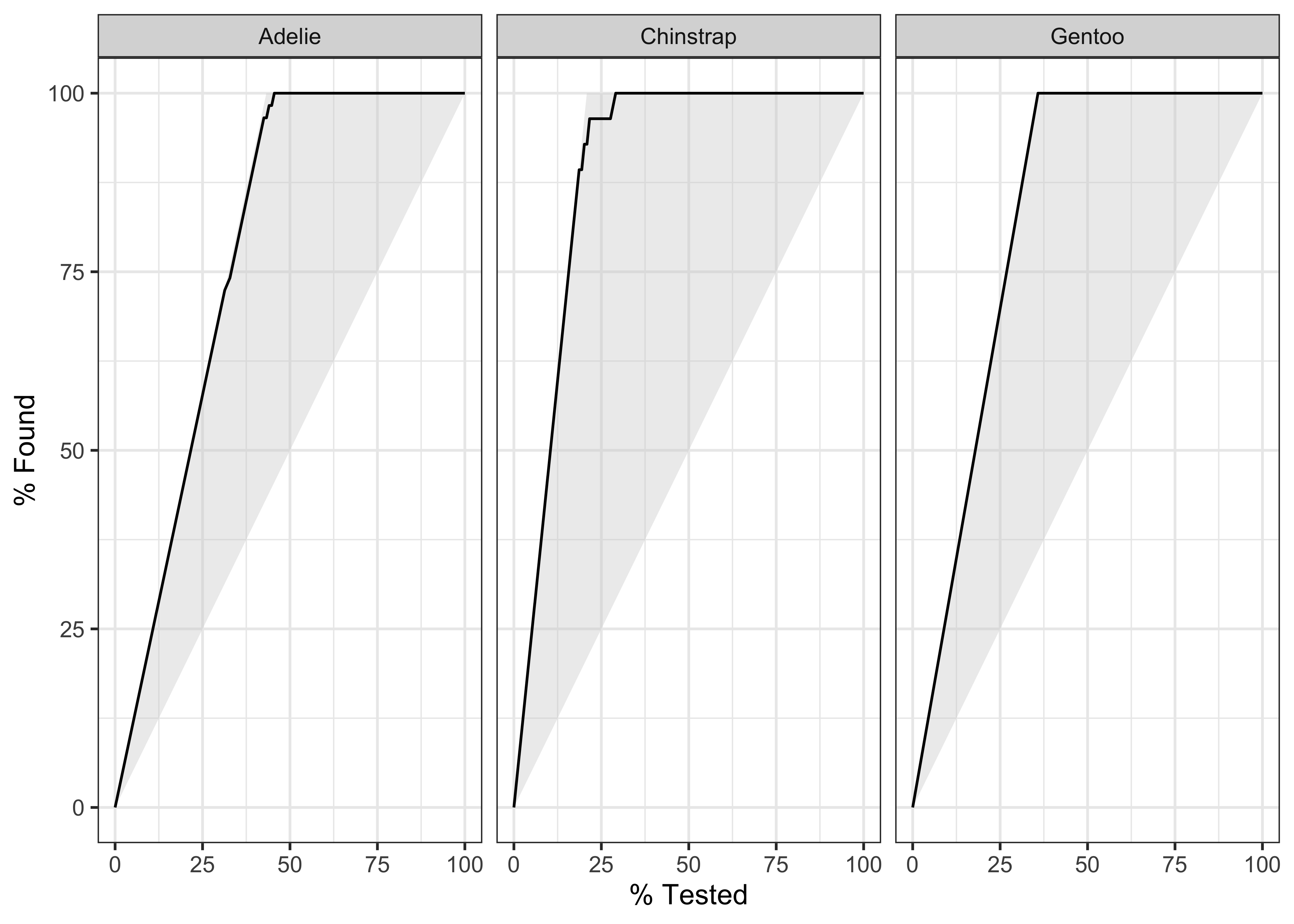

Using `broom` on the penguin model

penguin_split

<Training/Testing/Total>
<199/134/333>

penguin_split %>% broom::tidy()

penguin_recipe %>% broom::tidy()

# Following do not work for `random forest models` !! ;-()
# penguin_model %>% tidy()
# penguin_fit %>% tidy()
penguin_model %>% str()

List of 7
 $ args                 :List of 3
  ..$ mtry : language ~NULL
  .. ..- attr(*, ".Environment")=<environment: R_EmptyEnv> 
  ..$ trees: language ~100
  .. ..- attr(*, ".Environment")=<environment: R_EmptyEnv> 
  ..$ min_n: language ~NULL
  .. ..- attr(*, ".Environment")=<environment: R_EmptyEnv> 
 $ eng_args             : Named list()
  ..- attr(*, "class")= chr [1:2] "quosures" "list"
 $ mode                 : chr "classification"
 $ user_specified_mode  : logi TRUE
 $ method               : NULL
 $ engine               : chr "randomForest"
 $ user_specified_engine: logi TRUE
 - attr(*, "class")= chr [1:2] "rand_forest" "model_spec"

penguin_test_baked

Iris Random Forest Model with `ranger`

Using the iris dataset and Random Forest Classification. This part uses rsample to split the data and the recipes to prep the data for model making.

# set.seed(100)
iris_split <- rsample::initial_split(iris, prop = 0.6)
iris_split

<Training/Testing/Total>
<90/60/150>

iris_split %>%
  training() %>%
  glimpse()

Rows: 90
Columns: 5
$ Sepal.Length <dbl> 7.2, 5.1, 6.7, 6.7, 7.1, 5.0, 5.1, 5.2, 6.0, 5.9, 6.6, 5.…
$ Sepal.Width  <dbl> 3.6, 3.8, 3.0, 3.1, 3.0, 3.5, 3.5, 2.7, 2.2, 3.0, 2.9, 3.…
$ Petal.Length <dbl> 6.1, 1.5, 5.2, 4.4, 5.9, 1.6, 1.4, 3.9, 5.0, 4.2, 4.6, 1.…
$ Petal.Width  <dbl> 2.5, 0.3, 2.3, 1.4, 2.1, 0.6, 0.2, 1.4, 1.5, 1.5, 1.3, 0.…
$ Species      <fct> virginica, setosa, virginica, versicolor, virginica, seto…

iris_split %>%
  testing() %>%
  glimpse()

Rows: 60
Columns: 5
$ Sepal.Length <dbl> 4.6, 5.4, 4.4, 4.8, 4.8, 5.7, 4.6, 4.8, 5.0, 5.2, 4.8, 5.…
$ Sepal.Width  <dbl> 3.1, 3.9, 2.9, 3.4, 3.0, 3.8, 3.6, 3.4, 3.4, 3.4, 3.1, 3.…
$ Petal.Length <dbl> 1.5, 1.7, 1.4, 1.6, 1.4, 1.7, 1.0, 1.9, 1.6, 1.4, 1.6, 1.…
$ Petal.Width  <dbl> 0.2, 0.4, 0.2, 0.2, 0.1, 0.3, 0.2, 0.2, 0.4, 0.2, 0.2, 0.…
$ Species      <fct> setosa, setosa, setosa, setosa, setosa, setosa, setosa, s…

Iris Data Pre-Processing: Creating the Recipe

The recipes package provides an interface that specializes in data pre-processing. Within the package, the functions that start, or execute, the data transformations are named after cooking actions. That makes the interface more user-friendly. For example:

recipe() - Starts a new set of transformations to be applied, similar to the ggplot() command. Its main argument is the model’s formula.
prep() - Executes the transformations on top of the data that is supplied (typically, the training data). Each data transformation is a step() function. ( Recall what we did with the caret package: Centering, Scaling, Removing Correlated variables…)

Note that in order to avoid data leakage (e.g: transferring information from the train set into the test set), data should be “prepped” using the train_tbl only. https://towardsdatascience.com/modelling-with-tidymodels-and-parsnip-bae2c01c131c CRAN: The idea is that the preprocessing operations will all be created using the training set and then these steps will be applied to both the training and test set.

# Pre Processing the Training Data

iris_recipe <-
  training(iris_split) %>% # Note: Using TRAINING data !!
  recipe(Species ~ .) # Note: Outcomes ~ Predictors !!

# The data contained in the `data` argument need not be the training set; this data is only used to catalog the names of the variables and their types (e.g. numeric, etc.).

Q: How does the recipe “figure” out which are the outcomes and which are the predictors? A.The recipe command defines Outcomes and Predictors using the formula interface. ~~Not clear how this recipe “figures” out which are the outcomes and which are the predictors, when we have not yet specified them…~~

Q. Why is the recipe not agnostic to data set? Is that a meaningful question? A. The use of the training set in the recipe command is just to declare the variables and specify the roles of the data, nothing else. Roles are open-ended and extensible. From https://cran.r-project.org/web/packages/recipes/vignettes/Simple_Example.html :

This document demonstrates some basic uses of recipes. First, some definitions are required: - variables are the original (raw) data columns in a data frame or tibble. For example, in a traditional formula Y ~ A + B + A:B, the variables are A, B, and Y. - roles define how variables will be used in the model. Examples are: predictor (independent variables), response, and case weight. This is meant to be open-ended and extensible. - terms are columns in a design matrix such as A, B, and A:B. These can be other derived entities that are grouped, such as a set of principal components or a set of columns, that define a basis function for a variable. These are synonymous with features in machine learning. Variables that have predictor roles would automatically be main effect terms.

# Apply the transformation steps
iris_recipe <- iris_recipe %>%
  step_corr(all_predictors()) %>%
  step_center(all_predictors(), -all_outcomes()) %>%
  step_scale(all_predictors(), -all_outcomes()) %>%
  prep()

This has created the recipe() and prepped it too. We now need to apply it to our datasets:

Take training data and bake() it to prepare it for modelling.
Do the same for the testing set.

iris_training_baked <-
  iris_split %>%
  training() %>%
  bake(iris_recipe, .)
iris_training_baked

iris_testing_baked <-
  iris_split %>%
  testing() %>%
  bake(iris_recipe, .)
iris_testing_baked

Iris Model Training using `parsnip`

Different ML packages provide different interfaces (APIs ) to do the same thing (e.g random forests). The tidymodels package provides a consistent interface to invoke a wide variety of packages supporting a wide variety of models.

The parsnip package is a successor to caret.

To model with parsnip: 1. Pick a model : 2. Set the engine 3. Set the mode (if needed): Classification or Regression

Check here for models available in parsnip.

Mode: classification and regression in parsnip, each using a variety of models. ( Which Way). This defines the form of the output.
Engine: The engine is the R package that is invoked by parsnip to execute the model. E.g glm, glmnet,keras.( How ) parsnip provides wrappers for models from these packages.
Model: is the specific technique used for the modelling task. E.g linear_reg(), logistic_reg(), mars, decision_tree, nearest_neighbour…(What model).

and models have: - hyperparameters: that are numerical or factor variables that tune the model ( Like the alpha beta parameters for Bayesian priors)

We can use the random forest model to classify the iris into species. Here Species is the Outcome variable and the rest are predictor variables. The random forest model is provided by the ranger package, to which tidymodels/parsnip provides a simple and consistent interface.

library(ranger)
iris_ranger <-
  rand_forest(trees = 100) %>%
  set_mode("classification") %>%
  set_engine("ranger") %>%
  fit(Species ~ ., data = iris_training_baked)

ranger can generate random forest models for classification, regression, survival( time series, time to event stuff). Extreme Forests are also supported, wherein all points in the dataset are used ( instead of bootstrap samples) along with feature bagging. We can also run the same model using the randomForest package:

library(randomForest, quietly = TRUE)
iris_rf <-
  rand_forest(trees = 100) %>%
  set_mode("classification") %>%
  set_engine("randomForest") %>%
  fit(Species ~ ., data = iris_training_baked)

Iris Predictions

The predict() function run against a parsnip model returns a prediction tibble. By default, the prediction variable is called .pred_class.

predict(object = iris_ranger, new_data = iris_testing_baked) %>%
  dplyr::bind_cols(iris_testing_baked) %>%
  glimpse()

Rows: 60
Columns: 5
$ .pred_class  <fct> setosa, setosa, setosa, setosa, setosa, setosa, setosa, s…
$ Sepal.Length <dbl> -1.5852786, -0.5918925, -1.8336251, -1.3369321, -1.336932…
$ Sepal.Width  <dbl> 0.05284097, 1.78218168, -0.37949421, 0.70134373, -0.16332…
$ Petal.Width  <dbl> -1.3124100, -1.0448745, -1.3124100, -1.3124100, -1.446177…
$ Species      <fct> setosa, setosa, setosa, setosa, setosa, setosa, setosa, s…

Iris Classification Model Validation

We use metrics() function from the yardstick package to evaluate how good the model is.

predict(iris_ranger, iris_testing_baked) %>%
  dplyr::bind_cols(iris_testing_baked) %>%
  yardstick::metrics(truth = Species, estimate = .pred_class)

We can also check the metrics for randomForest model:

predict(iris_rf, iris_testing_baked) %>%
  dplyr::bind_cols(iris_testing_baked) %>%
  yardstick::metrics(truth = Species, estimate = .pred_class)

Iris Per-Classifier Metrics

We can use the parameter type = "prob" in the predict() function to obtain a probability score on each prediction. TBD: How is this prob calculated? Possible answer: the Random Forest model outputs its answer by majority voting across n trees. Each of the possible answers( i.e. predictions) for a particular test datum gets a share of the vote, that represents its probability. Hence each dataum in the test vector can show a probability for the “winning” answer. ( Quite possibly we can get the probabilities for all possible outcomes for each test datum)

iris_ranger_probs <-
  predict(iris_ranger, iris_testing_baked, type = "prob") %>%
  dplyr::bind_cols(iris_testing_baked)
glimpse(iris_ranger_probs)

Rows: 60
Columns: 7
$ .pred_setosa     <dbl> 0.980329365, 0.980809524, 0.887333333, 0.964476190, 0…
$ .pred_versicolor <dbl> 0.01967063, 0.00900000, 0.10541667, 0.02385714, 0.014…
$ .pred_virginica  <dbl> 0.000000000, 0.010190476, 0.007250000, 0.011666667, 0…
$ Sepal.Length     <dbl> -1.5852786, -0.5918925, -1.8336251, -1.3369321, -1.33…
$ Sepal.Width      <dbl> 0.05284097, 1.78218168, -0.37949421, 0.70134373, -0.1…
$ Petal.Width      <dbl> -1.3124100, -1.0448745, -1.3124100, -1.3124100, -1.44…
$ Species          <fct> setosa, setosa, setosa, setosa, setosa, setosa, setos…

iris_rf_probs <-
  predict(iris_rf, iris_testing_baked, type = "prob") %>%
  dplyr::bind_cols(iris_testing_baked)
glimpse(iris_rf_probs)

Rows: 60
Columns: 7
$ .pred_setosa     <dbl> 1.00, 1.00, 0.94, 0.99, 1.00, 0.87, 0.99, 0.99, 0.99,…
$ .pred_versicolor <dbl> 0.00, 0.00, 0.06, 0.00, 0.00, 0.10, 0.00, 0.00, 0.00,…
$ .pred_virginica  <dbl> 0.00, 0.00, 0.00, 0.01, 0.00, 0.03, 0.01, 0.01, 0.01,…
$ Sepal.Length     <dbl> -1.5852786, -0.5918925, -1.8336251, -1.3369321, -1.33…
$ Sepal.Width      <dbl> 0.05284097, 1.78218168, -0.37949421, 0.70134373, -0.1…
$ Petal.Width      <dbl> -1.3124100, -1.0448745, -1.3124100, -1.3124100, -1.44…
$ Species          <fct> setosa, setosa, setosa, setosa, setosa, setosa, setos…

# Tabulating the probabilities
ftable(iris_rf_probs$.pred_versicolor)

  0 0.01 0.02 0.03 0.04 0.05 0.06 0.08 0.1 0.18 0.2 0.24 0.27 0.3 0.33 0.43 0.59 0.61 0.63 0.7 0.71 0.8 0.83 0.84 0.86 0.9 0.91 0.93 0.94  1
                                                                                                                                            
 16    3    1    4    1    1    4    2   3    1   1    1    1   2    1    1    2    1    1   1    1   1    2    1    1   1    1    2    1  1

ftable(iris_rf_probs$.pred_virginica)

  0 0.01 0.03 0.05 0.06 0.07 0.08 0.09 0.14 0.16 0.17 0.19 0.29 0.37 0.41 0.57 0.67 0.69 0.7 0.73 0.75 0.79 0.82 0.9 0.92 0.94 0.95 0.97 0.99  1
                                                                                                                                                
 14    7    1    2    1    2    1    1    1    1    1    1    1    2    1    1    1    1   1    1    1    1    1   2    2    5    1    1    3  1

ftable(iris_rf_probs$.pred_setosa)

  0 0.01 0.03 0.04 0.05 0.1 0.2 0.24 0.87 0.94 0.95 0.96 0.98 0.99  1
                                                                     
 23    9    2    1    1   1   2    1    1    2    1    1    1    5  9

Iris Classifier: Gain and ROC Curves

We can plot gain and ROC curves for each of these models

iris_ranger_probs %>%
  yardstick::gain_curve(Species, .pred_setosa:.pred_virginica) %>%
  glimpse()

Rows: 145
Columns: 5
$ .level          <chr> "setosa", "setosa", "setosa", "setosa", "setosa", "set…
$ .n              <dbl> 0, 1, 3, 4, 6, 7, 9, 10, 12, 13, 14, 15, 16, 17, 18, 1…
$ .n_events       <dbl> 0, 1, 3, 4, 6, 7, 9, 10, 12, 13, 14, 15, 16, 17, 18, 1…
$ .percent_tested <dbl> 0.000000, 1.666667, 5.000000, 6.666667, 10.000000, 11.…
$ .percent_found  <dbl> 0, 5, 15, 20, 30, 35, 45, 50, 60, 65, 70, 75, 80, 85, …

iris_ranger_probs %>%
  yardstick::gain_curve(Species, .pred_setosa:.pred_virginica) %>%
  autoplot()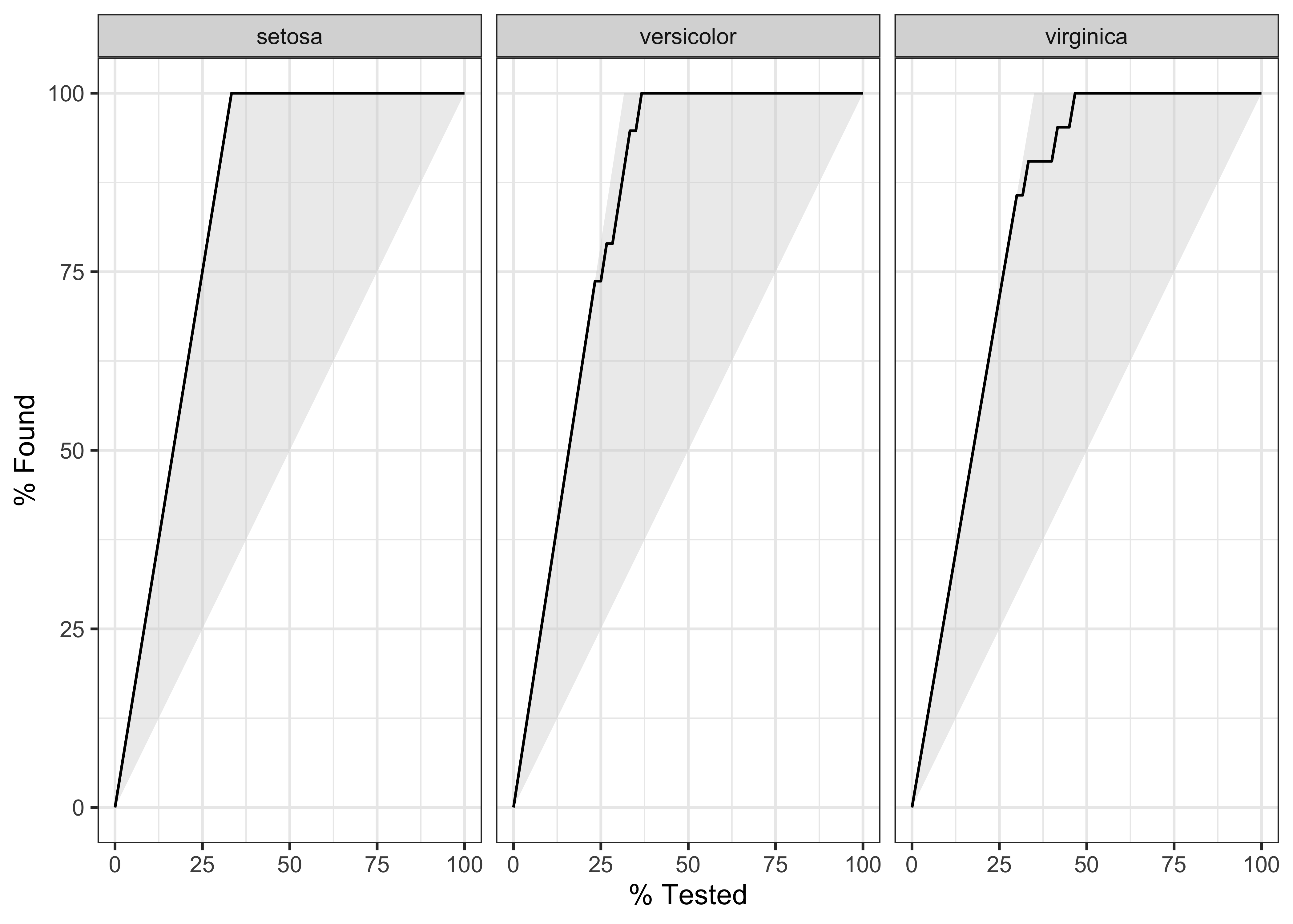

iris_ranger_probs %>%
  yardstick::roc_curve(Species, .pred_setosa:.pred_virginica) %>%
  glimpse()

Rows: 148
Columns: 4
$ .level      <chr> "setosa", "setosa", "setosa", "setosa", "setosa", "setosa"…
$ .threshold  <dbl> -Inf, 0.000000000, 0.001111111, 0.002000000, 0.002361111, …
$ specificity <dbl> 0.000, 0.000, 0.225, 0.275, 0.300, 0.325, 0.375, 0.500, 0.…
$ sensitivity <dbl> 1, 1, 1, 1, 1, 1, 1, 1, 1, 1, 1, 1, 1, 1, 1, 1, 1, 1, 1, 1…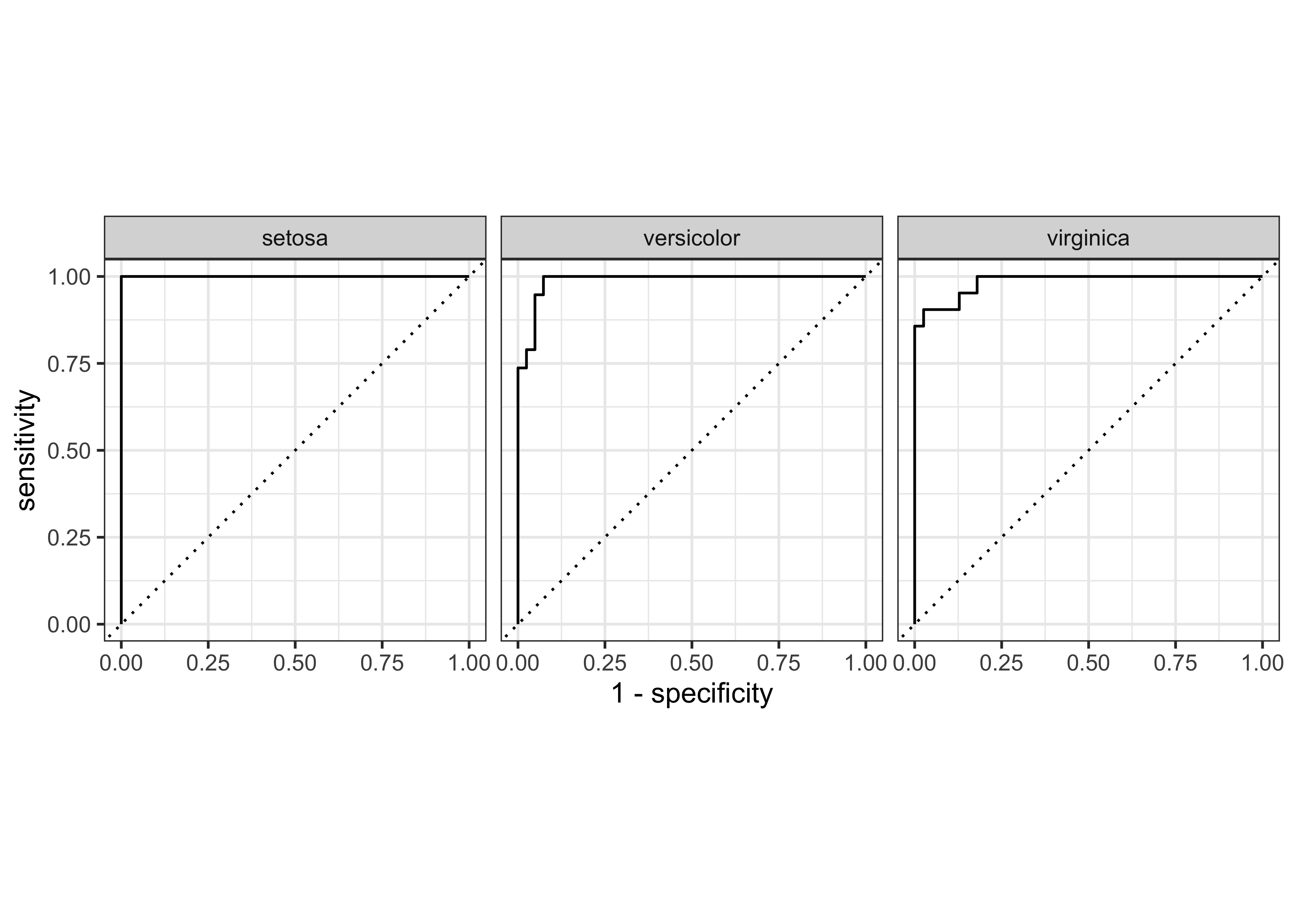

iris_ranger_probs %>%
  yardstick::roc_curve(Species, .pred_setosa:.pred_virginica) %>%
  autoplot()

iris_rf_probs %>%
  yardstick::gain_curve(Species, .pred_setosa:.pred_virginica) %>%
  glimpse()

Rows: 78
Columns: 5
$ .level          <chr> "setosa", "setosa", "setosa", "setosa", "setosa", "set…
$ .n              <dbl> 0, 9, 14, 15, 16, 17, 19, 20, 21, 23, 24, 25, 26, 28, …
$ .n_events       <dbl> 0, 9, 14, 15, 16, 17, 19, 20, 20, 20, 20, 20, 20, 20, …
$ .percent_tested <dbl> 0.000000, 15.000000, 23.333333, 25.000000, 26.666667, …
$ .percent_found  <dbl> 0.000000, 45.000000, 70.000000, 75.000000, 80.000000, …

iris_rf_probs %>%
  yardstick::gain_curve(Species, .pred_setosa:.pred_virginica) %>%
  autoplot()

iris_rf_probs %>%
  yardstick::roc_curve(Species, .pred_setosa:.pred_virginica) %>%
  glimpse()

Rows: 81
Columns: 4
$ .level      <chr> "setosa", "setosa", "setosa", "setosa", "setosa", "setosa"…
$ .threshold  <dbl> -Inf, 0.00, 0.01, 0.03, 0.04, 0.05, 0.10, 0.20, 0.24, 0.87…
$ specificity <dbl> 0.0000000, 0.0000000, 0.5750000, 0.8000000, 0.8500000, 0.8…
$ sensitivity <dbl> 1.00, 1.00, 1.00, 1.00, 1.00, 1.00, 1.00, 1.00, 1.00, 1.00…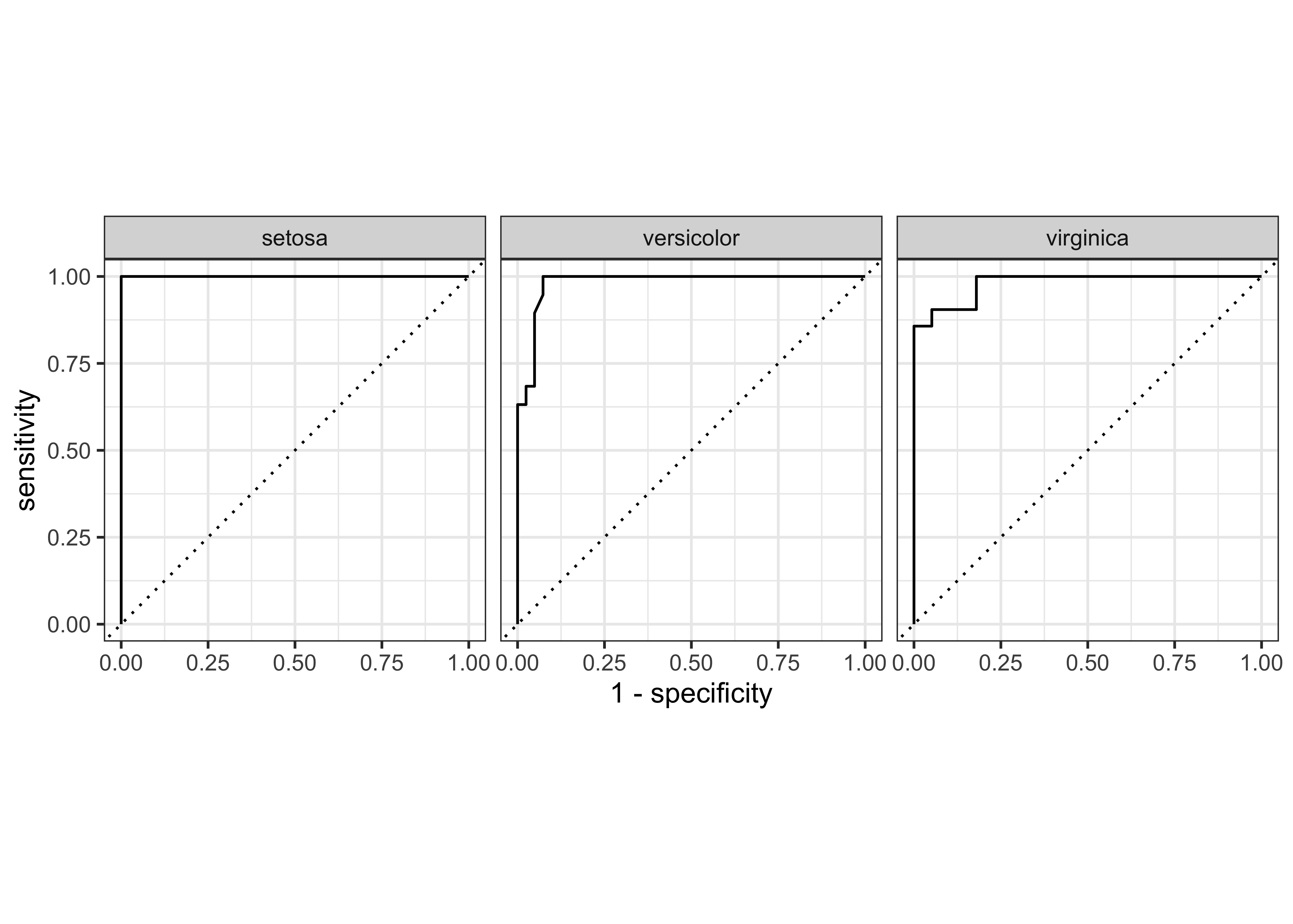

iris_rf_probs %>%
  yardstick::roc_curve(Species, .pred_setosa:.pred_virginica) %>%
  autoplot()

Iris Classifier: Metrics

predict(iris_ranger, iris_testing_baked, type = "prob") %>%
  bind_cols(predict(iris_ranger, iris_testing_baked)) %>%
  bind_cols(select(iris_testing_baked, Species)) %>%
  glimpse()

Rows: 60
Columns: 5
$ .pred_setosa     <dbl> 0.980329365, 0.980809524, 0.887333333, 0.964476190, 0…
$ .pred_versicolor <dbl> 0.01967063, 0.00900000, 0.10541667, 0.02385714, 0.014…
$ .pred_virginica  <dbl> 0.000000000, 0.010190476, 0.007250000, 0.011666667, 0…
$ .pred_class      <fct> setosa, setosa, setosa, setosa, setosa, setosa, setos…
$ Species          <fct> setosa, setosa, setosa, setosa, setosa, setosa, setos…

# predict(iris_ranger, iris_testing_baked, type = "prob") %>%
#   bind_cols(predict(iris_ranger,iris_testing_baked)) %>%
#   bind_cols(select(iris_testing_baked,Species)) %>%
#   yardstick::metrics(data = ., truth = Species, estimate = .pred_class, ... = .pred_setosa:.pred_virginica)


# And for the `randomForest`method

predict(iris_rf, iris_testing_baked, type = "prob") %>%
  bind_cols(predict(iris_ranger, iris_testing_baked)) %>%
  bind_cols(select(iris_testing_baked, Species)) %>%
  glimpse()

Rows: 60
Columns: 5
$ .pred_setosa     <dbl> 1.00, 1.00, 0.94, 0.99, 1.00, 0.87, 0.99, 0.99, 0.99,…
$ .pred_versicolor <dbl> 0.00, 0.00, 0.06, 0.00, 0.00, 0.10, 0.00, 0.00, 0.00,…
$ .pred_virginica  <dbl> 0.00, 0.00, 0.00, 0.01, 0.00, 0.03, 0.01, 0.01, 0.01,…
$ .pred_class      <fct> setosa, setosa, setosa, setosa, setosa, setosa, setos…
$ Species          <fct> setosa, setosa, setosa, setosa, setosa, setosa, setos…

# predict(iris_rf, iris_testing_baked, type = "prob") %>%
#   bind_cols(predict(iris_ranger,iris_testing_baked)) %>%
#   bind_cols(select(iris_testing_baked,Species)) %>%
#   yardstick::metrics(data = ., truth = Species, estimate = .pred_class, ... = .pred_setosa:.pred_virginica)

References

Machine Learning Basics - Random Forest at Shirin’s Playground

Penguin Random Forest Model withrandomForest

Penguin Data Sampling and Recipe

Penguin Random Forest Model

Metrics for the Penguin Random Forest Model

Using broom on the penguin model

Iris Random Forest Model with ranger

Iris Data Pre-Processing: Creating the Recipe

Iris Model Training using parsnip

Iris Predictions

Iris Classification Model Validation

Iris Per-Classifier Metrics

Iris Classifier: Gain and ROC Curves

Iris Classifier: Metrics

References

Penguin Random Forest Model with`randomForest`

Using `broom` on the penguin model

Iris Random Forest Model with `ranger`

Iris Model Training using `parsnip`