library(tidyverse)
library(mosaic)
library(ggformula)
library(ggridges)
library(skimr)
##
library(GGally)
library(corrplot)
library(corrgram)
library(crosstable) # Summary stats tables
library(kableExtra)
##
library(paletteer) # Colour Palettes for Peasants
##
## Add other packages here as needed, e.g.:
## scales/ggprism;
## ggstats/correlation;
## vcd/vcdExtra/ggalluvial/ggpubr;
## sf/tmap/osmplotr/rnaturalearth;
## igraph/tidygraph/ggraph/graphlayouts;
EDA
Workflow
Descriptive
Abstract
A complete EDA Workflow
A Data Analytics Process
So you have your shiny new R skills and you’ve successfully loaded a cool dataframe into R… Now what?
The best charts come from understanding your data, asking good questions from it, and displaying the answers to those questions as clearly as possible.
- Create a new Project in RStudio. File -> New Project -> Quarto Blog
- Create a new Quarto document: all your Quarto documents should be in the
posts/folder. See the samples therein to get an idea. - Save the document with a meaningful name, e.g.
EDA-Workflow.qmd - Create a new folder in the Project for your data files, e.g.
data/. This can be at the inside theposts/folder. - Store all datasets within this folder, and refer to them with relative paths, e.g.
../data/mydata.csvin any other Quarto document in the Project. (../means “go up one level from the current folder”.)
Now edit the `.qmd file which you are editing for this report to include the following sections, YAML, code chunks, and text as needed.
Download this document as a Work Template
Hit the </>Code button at upper right to copy/save this very document as a Quarto Markdown template for your work. Delete the text that you don’t need, but keep most of the Sections as they are!
- Install packages using
install.packages()in your Console. - Load up your libraries in a
setupchunk: - Add
knitroptions to your YAML header, so that all your plots are rendered in high quality PNG format.
title: "My Document"
format: html
knitr:
  opts_chunk:
    dev: "ragg_png"
Set up a theme for your plots. This is a good time to set up your own theme, or use an existing one, e.g. ggprism, ggthemes, ggpubr, etc. If you have a Company logo, you can use that as a theme too.
Show the Code
# Chunk options
knitr::opts_chunk$set(
  fig.width = 7,
  fig.asp = 0.618, # Golden Ratio
  # out.width = "80%",
  fig.align = "center"
)
### Ggplot Theme
### https://rpubs.com/mclaire19/ggplot2-custom-themes
### https://stackoverflow.com/questions/74491138/ggplot-custom-fonts-not-working-in-quarto

# We have locally downloaded the `Alegreya` and `Roboto Condensed` fonts.
# This ensures we are GDPR-compliant, and not using Google Fonts directly.
# Let us import these local fonts into our session and use them to define our ggplot theme.
library(sysfonts)

sysfonts::font_add(
  family = "Alegreya",
  regular = "../../../../../../fonts/Alegreya-Regular.ttf",
  italic = "../../../../../../fonts/Alegreya-Italic.ttf",
  bold = "../../../../../../fonts/Alegreya-Bold.ttf",
  bolditalic = "../../../../../../fonts/Alegreya-BoldItalic.ttf"
)

sysfonts::font_add(
  family = "Roboto Condensed",
  regular = "../../../../../../fonts/RobotoCondensed-Regular.ttf",
  italic = "../../../../../../fonts/RobotoCondensed-Italic.ttf",
  bold = "../../../../../../fonts/RobotoCondensed-Bold.ttf",
  bolditalic = "../../../../../../fonts/RobotoCondensed-BoldItalic.ttf"
)


theme_custom <- function() {
  font <- "Alegreya" # assign font family up front

  theme_classic(base_size = 14) %+replace% # replace elements we want to change

    theme(
      text = element_text(family = "Alegreya"), # set default font family for all text

      # text elements
      plot.title = element_text( # title
        family = "Alegreya", # set font family
        size = 18, # set font size
        face = "bold", # bold typeface
        hjust = 0, # left align
        vjust = 2
      ), # raise slightly

      plot.title.position = "plot",
      plot.subtitle = element_text( # subtitle
        family = "Alegreya", # font family
        size = 14
      ), # font size

      plot.caption = element_text( # caption
        family = "Alegreya", # font family
        size = 9, # font size
        hjust = 1
      ), # right align

      plot.caption.position = "plot", # right align

      axis.title = element_text( # axis titles
        family = "Roboto Condensed", # font family
        size = 10
      ), # font size

      axis.text = element_text( # axis text
        family = "Roboto Condensed", # font family
        size = 9
      ), # font size

      axis.text.x = element_text( # margin for axis text
        margin = margin(5, b = 10)
      )

      # since the legend often requires manual tweaking
      # based on plot content, don't define it here
    )
}

## Use available fonts in ggplot text geoms too!
update_geom_defaults(geom = "text", new = list(
  family = "Roboto Condensed",
  face = "plain",
  size = 3.5,
  color = "#2b2b2b"
))

## Set the theme
theme_set(new = theme_custom())
Use Namespace based Code
Warning
Try always to name your code-command with the package from whence it came! So use dplyr::filter() / dplyr::summarize() and not just filter() or summarize(), since these commands could exist across multiple packages, which you may have loaded last.
(One can also use the conflicted package to set this up, but this is simpler for beginners like us. )
- Use
readr::read_csv(); ordata(...)if the data is in a package
data(penguins, package = "palmerpenguins")
- Use
dplyr::glimpse() - Use
mosaic::inspect()orskimr::skim() - Use
dplyr::summarise()andcrosstable::crosstable() - Format your tables with
knitr::kable() - Highlight any interesting summary stats or data imbalances
dplyr::glimpse(penguins)Rows: 344
Columns: 8
$ species <fct> Adelie, Adelie, Adelie, Adelie, Adelie, Adelie, Adel…
$ island <fct> Torgersen, Torgersen, Torgersen, Torgersen, Torgerse…
$ bill_length_mm <dbl> 39.1, 39.5, 40.3, NA, 36.7, 39.3, 38.9, 39.2, 34.1, …
$ bill_depth_mm <dbl> 18.7, 17.4, 18.0, NA, 19.3, 20.6, 17.8, 19.6, 18.1, …
$ flipper_length_mm <int> 181, 186, 195, NA, 193, 190, 181, 195, 193, 190, 186…
$ body_mass_g <int> 3750, 3800, 3250, NA, 3450, 3650, 3625, 4675, 3475, …
$ sex <fct> male, female, female, NA, female, male, female, male…
$ year <int> 2007, 2007, 2007, 2007, 2007, 2007, 2007, 2007, 2007…skimr::skim(penguins)| Name | penguins |
| Number of rows | 344 |
| Number of columns | 8 |
| _______________________ | |
| Column type frequency: | |
| factor | 3 |
| numeric | 5 |
| ________________________ | |
| Group variables | None |
Variable type: factor
| skim_variable | n_missing | complete_rate | ordered | n_unique | top_counts |
|---|---|---|---|---|---|
| species | 0 | 1.00 | FALSE | 3 | Ade: 152, Gen: 124, Chi: 68 |
| island | 0 | 1.00 | FALSE | 3 | Bis: 168, Dre: 124, Tor: 52 |
| sex | 11 | 0.97 | FALSE | 2 | mal: 168, fem: 165 |
Variable type: numeric
| skim_variable | n_missing | complete_rate | mean | sd | p0 | p25 | p50 | p75 | p100 | hist |
|---|---|---|---|---|---|---|---|---|---|---|
| bill_length_mm | 2 | 0.99 | 43.92 | 5.46 | 32.1 | 39.23 | 44.45 | 48.5 | 59.6 | ▃▇▇▆▁ |
| bill_depth_mm | 2 | 0.99 | 17.15 | 1.97 | 13.1 | 15.60 | 17.30 | 18.7 | 21.5 | ▅▅▇▇▂ |
| flipper_length_mm | 2 | 0.99 | 200.92 | 14.06 | 172.0 | 190.00 | 197.00 | 213.0 | 231.0 | ▂▇▃▅▂ |
| body_mass_g | 2 | 0.99 | 4201.75 | 801.95 | 2700.0 | 3550.00 | 4050.00 | 4750.0 | 6300.0 | ▃▇▆▃▂ |
| year | 0 | 1.00 | 2008.03 | 0.82 | 2007.0 | 2007.00 | 2008.00 | 2009.0 | 2009.0 | ▇▁▇▁▇ |
- Data Dictionary: A table containing the variable names, their interpretation, and their nature(Qual/Quant/Ord…)
- If there are wrongly coded variables in the original data, state them in their correct form, so you can munge the in the next step
- Declare what might be target and predictor variables, based on available information of the experiment, or a description of the data.
Qualitative Variables
- Categorical variables, e.g.
species,island,sex - Use
dplyr::count()to get counts of each category
Quantitative Variables
- Continuous variables, e.g.
body_mass_g,flipper_length_mm,bill_length_mm - Use
dplyr::summarise()to get summary statistics of each variable
- Convert variables to factors as needed
- Reformat / Rename other variables as needed
- Clean badly formatted columns (e.g. text + numbers) using
tidyr::separate_**_**() - Save the data as a modified file
- Do not mess up the original data file
```{r}
#| label: data-munging
#| eval: false

dataset_modified <- data %>%
  dplyr::mutate(across(where(is.character), as.factor))
# And so on
```
Munge the variables separately if you need to specify factor labels and levels for each variable.
Question-1
- State the Question or Hypothesis
- (Temporarily) Drop variables using
dplyr::select() - Create new variables if needed with
dplyr::mutate() - Filter the data set using
dplyr::filter() - Reformat data if needed with
tidyr::pivot_longer()ortidyr::pivot_wider() - Answer the Question with a Table, a Chart, a Test, using an appropriate Model for Statistical Inference
- Use
title,subtitle,legendandscalesappropriately in your chart - Prefer
ggformulaunless you are using a chart that is not yet supported therein (eg.ggbump()orplot_likert())
## Set graph theme
## Idiotic that we have to repeat this every chunk
## Open issue in Quarto
theme_set(new = theme_custom())
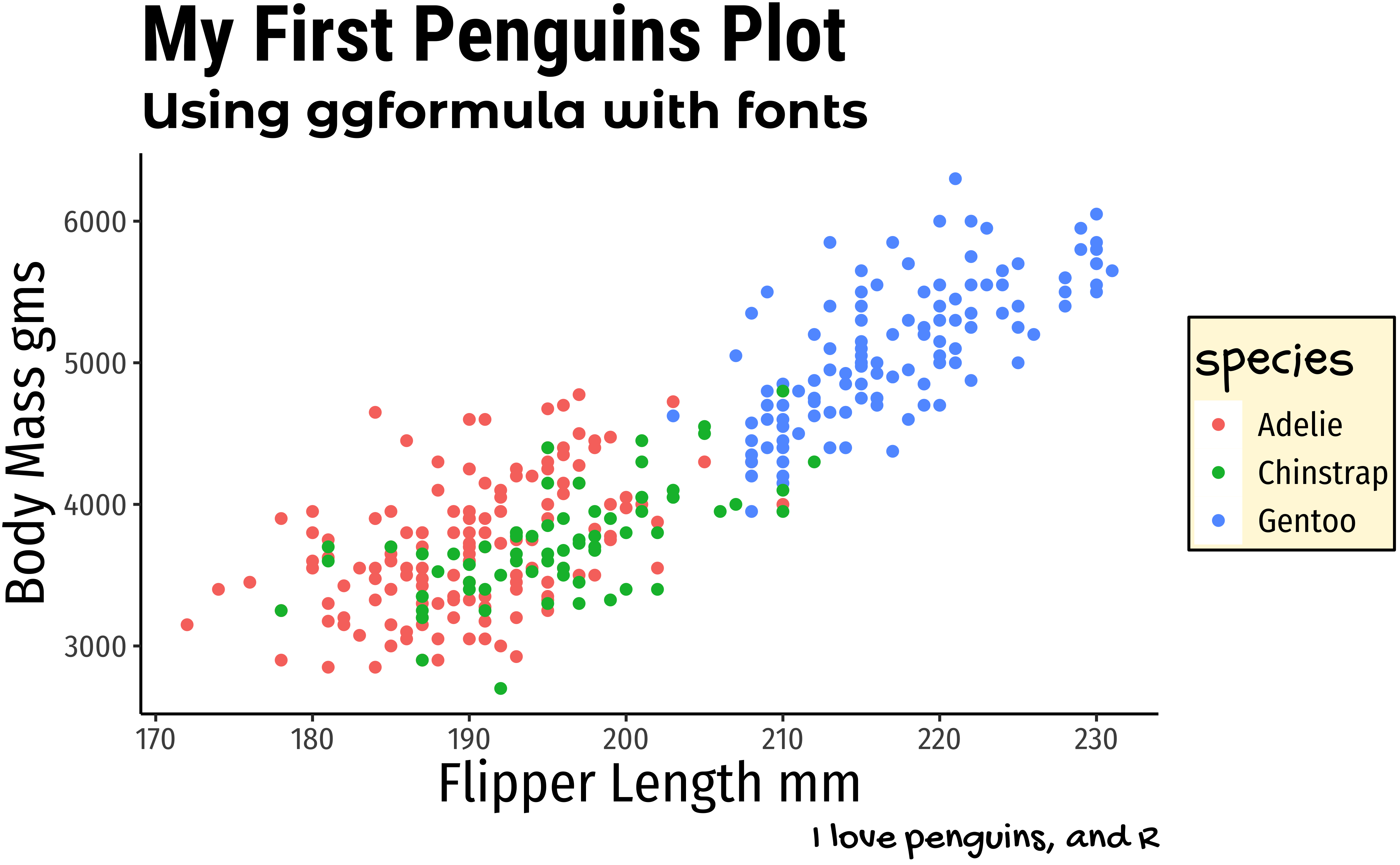
penguins %>%
tidyr::drop_na() %>%
gf_point(body_mass_g ~ flipper_length_mm,
colour = ~species
) %>%
gf_labs(
title = "My First Penguins Plot",
subtitle = "Using ggformula with fonts",
x = "Flipper Length mm", y = "Body Mass gms",
caption = "I love penguins, and R"
)
Inference-1
. . . .
Question-n
….
Inference-n
….
Describe what the graph shows and why it so interesting. What could be done next?
Over 2500 colour palettes are available in the paletteer package. Can you find tayloRswift? wesanderson? harrypotter? timburton? You could also find/define palettes that are in line with your Company’s logo / colour schemes.
Here are the Qualitative Palettes: (searchable)
And the Quantitative/Continuous palettes: (searchable)
Use the commands:
## For Qual variable-> colour/fill:
scale_colour_paletteer_d(
  name = "Legend Name",
  palette = "package::palette",
  dynamic = TRUE / FALSE
)

## For Quant variable-> colour/fill:
scale_colour_paletteer_c(
  name = "Legend Name",
  palette = "package::palette",
  dynamic = TRUE / FALSE
)