A Tidygraph version of a Popular Network Science Tutorial

R; Networks

Author

Arvind Venkatadri

Published

June 16, 2021

Modified

Invalid Date

Introduction

This is an attempt to rework , using tidygraph and ggraph, much of Network Visualization with R Polnet 2018 Workshop Tutorial, Washington, DC by Prof. Katherine (Katya) Ognyanova.

The aim is to get a working acquaintance with both these packages and also to appreciate some of the concepts in Networks. My code is by no means intended to be elegant; it merely works and there are surely many improvements that people may think of!

I have attempted to write code for the Sections 2:5. I have retained Prof. Ognyanova’s text in all places.

~~Working with colors in R plots~~
Reading in the network data
Network plots in ‘igraph’
Plotting two-mode networks
Plotting multiplex networks
~~Quick example using ‘network’~~
~~Simple plot animations in R~~
~~Interactive JavaScript networks~~
~~Interactive and dynamic networks with ndtv-d3~~
~~Plotting networks on a geographic map~~

——- DATASET 1: edgelist ——-

# Read in the data:
nodes <- read.csv("./Dataset1-Media-Example-NODES.csv", header = T, as.is = T)
links <- read.csv("./Dataset1-Media-Example-EDGES.csv", header = T, as.is = T)

# Examine the data:
head(nodes)

ABCDEFGHIJ0123456789

	id <chr>	media <chr>	media.type <int>	type.label <chr>	audience.size <int>
1	s01	NY Times	1	Newspaper	20
2	s02	Washington Post	1	Newspaper	25
3	s03	Wall Street Journal	1	Newspaper	30
4	s04	USA Today	1	Newspaper	32
5	s05	LA Times	1	Newspaper	20
6	s06	New York Post	1	Newspaper	50

head(links)

ABCDEFGHIJ0123456789

	from <chr>	to <chr>	type <chr>	weight <int>
1	s01	s02	hyperlink	22
2	s01	s03	hyperlink	22
3	s01	s04	hyperlink	21
4	s01	s15	mention	20
5	s02	s01	hyperlink	23
6	s02	s03	hyperlink	21

Converting the data to an igraph object:

The graph_from_data_frame() function takes two data frames: ‘d’ and ‘vertices’. - ‘d’ describes the edges of the network - it should start with two columns containing the source and target node IDs for each network tie. - ‘vertices’ should start with a column of node IDs. It can be omitted. - Any additional columns in either data frame are interpreted as attributes.

NOTE: ID columns need not be numbers or integers!!

net <- graph_from_data_frame(d = links, vertices = nodes, directed = T)

# Examine the resulting object:
class(net)

[1] "igraph"

net

IGRAPH 3b8a1d2 DNW- 17 49 -- 
+ attr: name (v/c), media (v/c), media.type (v/n), type.label (v/c),
| audience.size (v/n), type (e/c), weight (e/n)
+ edges from 3b8a1d2 (vertex names):
 [1] s01->s02 s01->s03 s01->s04 s01->s15 s02->s01 s02->s03 s02->s09 s02->s10
 [9] s03->s01 s03->s04 s03->s05 s03->s08 s03->s10 s03->s11 s03->s12 s04->s03
[17] s04->s06 s04->s11 s04->s12 s04->s17 s05->s01 s05->s02 s05->s09 s05->s15
[25] s06->s06 s06->s16 s06->s17 s07->s03 s07->s08 s07->s10 s07->s14 s08->s03
[33] s08->s07 s08->s09 s09->s10 s10->s03 s12->s06 s12->s13 s12->s14 s13->s12
[41] s13->s17 s14->s11 s14->s13 s15->s01 s15->s04 s15->s06 s16->s06 s16->s17
[49] s17->s04

The description of an igraph object starts with four letters:
- D or U, for a directed or undirected graph - N for a named graph (where nodes have a name attribute) - W for a weighted graph (where edges have a weight attribute) -B for a bipartite (two-mode) graph (where nodes have a type attribute) The two numbers that follow (17 49) refer to the number of nodes and edges in the graph. The description also lists node & edge attributes.

We can access the nodes, edges, and their attributes:

E(net)

+ 49/49 edges from 3b8a1d2 (vertex names):
 [1] s01->s02 s01->s03 s01->s04 s01->s15 s02->s01 s02->s03 s02->s09 s02->s10
 [9] s03->s01 s03->s04 s03->s05 s03->s08 s03->s10 s03->s11 s03->s12 s04->s03
[17] s04->s06 s04->s11 s04->s12 s04->s17 s05->s01 s05->s02 s05->s09 s05->s15
[25] s06->s06 s06->s16 s06->s17 s07->s03 s07->s08 s07->s10 s07->s14 s08->s03
[33] s08->s07 s08->s09 s09->s10 s10->s03 s12->s06 s12->s13 s12->s14 s13->s12
[41] s13->s17 s14->s11 s14->s13 s15->s01 s15->s04 s15->s06 s16->s06 s16->s17
[49] s17->s04

V(net)

+ 17/17 vertices, named, from 3b8a1d2:
 [1] s01 s02 s03 s04 s05 s06 s07 s08 s09 s10 s11 s12 s13 s14 s15 s16 s17

E(net)$type

 [1] "hyperlink" "hyperlink" "hyperlink" "mention"   "hyperlink" "hyperlink"
 [7] "hyperlink" "hyperlink" "hyperlink" "hyperlink" "hyperlink" "hyperlink"
[13] "mention"   "hyperlink" "hyperlink" "hyperlink" "mention"   "mention"  
[19] "hyperlink" "mention"   "mention"   "hyperlink" "hyperlink" "mention"  
[25] "hyperlink" "hyperlink" "mention"   "mention"   "mention"   "hyperlink"
[31] "mention"   "hyperlink" "mention"   "mention"   "mention"   "hyperlink"
[37] "mention"   "hyperlink" "mention"   "hyperlink" "mention"   "mention"  
[43] "mention"   "hyperlink" "hyperlink" "hyperlink" "hyperlink" "mention"  
[49] "hyperlink"

V(net)$media

 [1] "NY Times"            "Washington Post"     "Wall Street Journal"
 [4] "USA Today"           "LA Times"            "New York Post"      
 [7] "CNN"                 "MSNBC"               "FOX News"           
[10] "ABC"                 "BBC"                 "Yahoo News"         
[13] "Google News"         "Reuters.com"         "NYTimes.com"        
[16] "WashingtonPost.com"  "AOL.com"

# Using tidygraph
tbl_graph(nodes, links, directed = TRUE) %>%
  activate(edges) %>%
  select(type)

# A tbl_graph: 17 nodes and 49 edges
#
# A directed multigraph with 1 component
#
# Edge Data: 49 × 3 (active)
    from    to type     
   <int> <int> <chr>    
 1     1     2 hyperlink
 2     1     3 hyperlink
 3     1     4 hyperlink
 4     1    15 mention  
 5     2     1 hyperlink
 6     2     3 hyperlink
 7     2     9 hyperlink
 8     2    10 hyperlink
 9     3     1 hyperlink
10     3     4 hyperlink
# ℹ 39 more rows
#
# Node Data: 17 × 5
  id    media               media.type type.label audience.size
  <chr> <chr>                    <int> <chr>              <int>
1 s01   NY Times                     1 Newspaper             20
2 s02   Washington Post              1 Newspaper             25
3 s03   Wall Street Journal          1 Newspaper             30
# ℹ 14 more rows

tbl_graph(nodes, links, directed = TRUE) %>%
  activate(nodes) %>%
  select(media)

# A tbl_graph: 17 nodes and 49 edges
#
# A directed multigraph with 1 component
#
# Node Data: 17 × 1 (active)
   media              
   <chr>              
 1 NY Times           
 2 Washington Post    
 3 Wall Street Journal
 4 USA Today          
 5 LA Times           
 6 New York Post      
 7 CNN                
 8 MSNBC              
 9 FOX News           
10 ABC                
11 BBC                
12 Yahoo News         
13 Google News        
14 Reuters.com        
15 NYTimes.com        
16 WashingtonPost.com 
17 AOL.com            
#
# Edge Data: 49 × 4
   from    to type      weight
  <int> <int> <chr>      <int>
1     1     2 hyperlink     22
2     1     3 hyperlink     22
3     1     4 hyperlink     21
# ℹ 46 more rows

Or find specific nodes and edges by attribute:(that returns objects of type vertex sequence / edge sequence)

V(net)[media == "BBC"]

+ 1/17 vertex, named, from 3b8a1d2:
[1] s11

E(net)[type == "mention"]

+ 20/49 edges from 3b8a1d2 (vertex names):
 [1] s01->s15 s03->s10 s04->s06 s04->s11 s04->s17 s05->s01 s05->s15 s06->s17
 [9] s07->s03 s07->s08 s07->s14 s08->s07 s08->s09 s09->s10 s12->s06 s12->s14
[17] s13->s17 s14->s11 s14->s13 s16->s17

# Using tidygraph
tbl_graph(nodes, links, directed = TRUE) %>%
  activate(nodes) %>%
  filter(media == "BBC")

# A tbl_graph: 1 nodes and 0 edges
#
# A rooted tree
#
# Node Data: 1 × 5 (active)
  id    media media.type type.label audience.size
  <chr> <chr>      <int> <chr>              <int>
1 s11   BBC            2 TV                    34
#
# Edge Data: 0 × 4
# ℹ 4 variables: from <int>, to <int>, type <chr>, weight <int>

tbl_graph(nodes, links, directed = TRUE) %>%
  activate(edges) %>%
  filter(type == "mention")

# A tbl_graph: 17 nodes and 20 edges
#
# A directed simple graph with 3 components
#
# Edge Data: 20 × 4 (active)
    from    to type    weight
   <int> <int> <chr>    <int>
 1     1    15 mention     20
 2     3    10 mention      2
 3     4     6 mention      1
 4     4    11 mention     22
 5     4    17 mention      2
 6     5     1 mention      1
 7     5    15 mention     21
 8     6    17 mention     21
 9     7     3 mention      1
10     7     8 mention     22
11     7    14 mention      4
12     8     7 mention     21
13     8     9 mention     23
14     9    10 mention     21
15    12     6 mention      2
16    12    14 mention     22
17    13    17 mention      1
18    14    11 mention      1
19    14    13 mention     21
20    16    17 mention     21
#
# Node Data: 17 × 5
  id    media               media.type type.label audience.size
  <chr> <chr>                    <int> <chr>              <int>
1 s01   NY Times                     1 Newspaper             20
2 s02   Washington Post              1 Newspaper             25
3 s03   Wall Street Journal          1 Newspaper             30
# ℹ 14 more rows

If you need them, you can extract an edge list or a matrix back from the igraph networks.

as_edgelist(net, names = T)

      [,1]  [,2] 
 [1,] "s01" "s02"
 [2,] "s01" "s03"
 [3,] "s01" "s04"
 [4,] "s01" "s15"
 [5,] "s02" "s01"
 [6,] "s02" "s03"
 [7,] "s02" "s09"
 [8,] "s02" "s10"
 [9,] "s03" "s01"
[10,] "s03" "s04"
[11,] "s03" "s05"
[12,] "s03" "s08"
[13,] "s03" "s10"
[14,] "s03" "s11"
[15,] "s03" "s12"
[16,] "s04" "s03"
[17,] "s04" "s06"
[18,] "s04" "s11"
[19,] "s04" "s12"
[20,] "s04" "s17"
[21,] "s05" "s01"
[22,] "s05" "s02"
[23,] "s05" "s09"
[24,] "s05" "s15"
[25,] "s06" "s06"
[26,] "s06" "s16"
[27,] "s06" "s17"
[28,] "s07" "s03"
[29,] "s07" "s08"
[30,] "s07" "s10"
[31,] "s07" "s14"
[32,] "s08" "s03"
[33,] "s08" "s07"
[34,] "s08" "s09"
[35,] "s09" "s10"
[36,] "s10" "s03"
[37,] "s12" "s06"
[38,] "s12" "s13"
[39,] "s12" "s14"
[40,] "s13" "s12"
[41,] "s13" "s17"
[42,] "s14" "s11"
[43,] "s14" "s13"
[44,] "s15" "s01"
[45,] "s15" "s04"
[46,] "s15" "s06"
[47,] "s16" "s06"
[48,] "s16" "s17"
[49,] "s17" "s04"

as_adjacency_matrix(net, attr = "weight")

17 x 17 sparse Matrix of class "dgCMatrix"

                                                     
s01  . 22 22 21 .  .  .  .  .  .  .  .  .  . 20  .  .
s02 23  . 21  . .  .  .  .  1  5  .  .  .  .  .  .  .
s03 21  .  . 22 1  .  .  4  .  2  1  1  .  .  .  .  .
s04  .  . 23  . .  1  .  .  .  . 22  3  .  .  .  .  2
s05  1 21  .  . .  .  .  .  2  .  .  .  .  . 21  .  .
s06  .  .  .  . .  1  .  .  .  .  .  .  .  .  . 21 21
s07  .  .  1  . .  .  . 22  . 21  .  .  .  4  .  .  .
s08  .  .  2  . .  . 21  . 23  .  .  .  .  .  .  .  .
s09  .  .  .  . .  .  .  .  . 21  .  .  .  .  .  .  .
s10  .  .  2  . .  .  .  .  .  .  .  .  .  .  .  .  .
s11  .  .  .  . .  .  .  .  .  .  .  .  .  .  .  .  .
s12  .  .  .  . .  2  .  .  .  .  .  . 22 22  .  .  .
s13  .  .  .  . .  .  .  .  .  .  . 21  .  .  .  .  1
s14  .  .  .  . .  .  .  .  .  .  1  . 21  .  .  .  .
s15 22  .  .  1 .  4  .  .  .  .  .  .  .  .  .  .  .
s16  .  .  .  . . 23  .  .  .  .  .  .  .  .  .  . 21
s17  .  .  .  4 .  .  .  .  .  .  .  .  .  .  .  .  .

# Using tidygraph
# No direct command seems available ...

# Or data frames describing nodes and edges:
igraph::as_data_frame(x = net, what = "edges")

ABCDEFGHIJ0123456789

	from <chr>	to <chr>	type <chr>	weight <int>
1	s01	s02	hyperlink	22
2	s01	s03	hyperlink	22
3	s01	s04	hyperlink	21
4	s01	s15	mention	20
5	s02	s01	hyperlink	23
6	s02	s03	hyperlink	21
7	s02	s09	hyperlink	1
8	s02	s10	hyperlink	5
9	s03	s01	hyperlink	21
10	s03	s04	hyperlink	22

igraph::as_data_frame(x = net, what = "vertices")

ABCDEFGHIJ0123456789

	name <chr>	media <chr>	media.type <int>	type.label <chr>	audience.size <int>
s01	s01	NY Times	1	Newspaper	20
s02	s02	Washington Post	1	Newspaper	25
s03	s03	Wall Street Journal	1	Newspaper	30
s04	s04	USA Today	1	Newspaper	32
s05	s05	LA Times	1	Newspaper	20
s06	s06	New York Post	1	Newspaper	50
s07	s07	CNN	2	TV	56
s08	s08	MSNBC	2	TV	34
s09	s09	FOX News	2	TV	60
s10	s10	ABC	2	TV	23

# Using tidygraph
tbl_graph(nodes, links, directed = TRUE) %>%
  activate(nodes) %>%
  as_tibble()

ABCDEFGHIJ0123456789

id <chr>	media <chr>	media.type <int>	type.label <chr>	audience.size <int>
s01	NY Times	1	Newspaper	20
s02	Washington Post	1	Newspaper	25
s03	Wall Street Journal	1	Newspaper	30
s04	USA Today	1	Newspaper	32
s05	LA Times	1	Newspaper	20
s06	New York Post	1	Newspaper	50
s07	CNN	2	TV	56
s08	MSNBC	2	TV	34
s09	FOX News	2	TV	60
s10	ABC	2	TV	23

tbl_graph(nodes, links, directed = TRUE) %>%
  activate(edges) %>%
  as_tibble()

ABCDEFGHIJ0123456789

from <int>	to <int>	type <chr>	weight <int>
1	2	hyperlink	22
1	3	hyperlink	22
1	4	hyperlink	21
1	15	mention	20
2	1	hyperlink	23
2	3	hyperlink	21
2	9	hyperlink	1
2	10	hyperlink	5
3	1	hyperlink	21
3	4	hyperlink	22

# You can also access the network matrix directly:
net[1, ]

s01 s02 s03 s04 s05 s06 s07 s08 s09 s10 s11 s12 s13 s14 s15 s16 s17 
  0  22  22  21   0   0   0   0   0   0   0   0   0   0  20   0   0

net[5, 7]

[1] 0

# Using tidygraph
# Does not seem possible, even with `as.matrix()`.
# Returns tibbles only as in the code chunk above

# First attempt to plot the graph:
plot(net) # not pretty!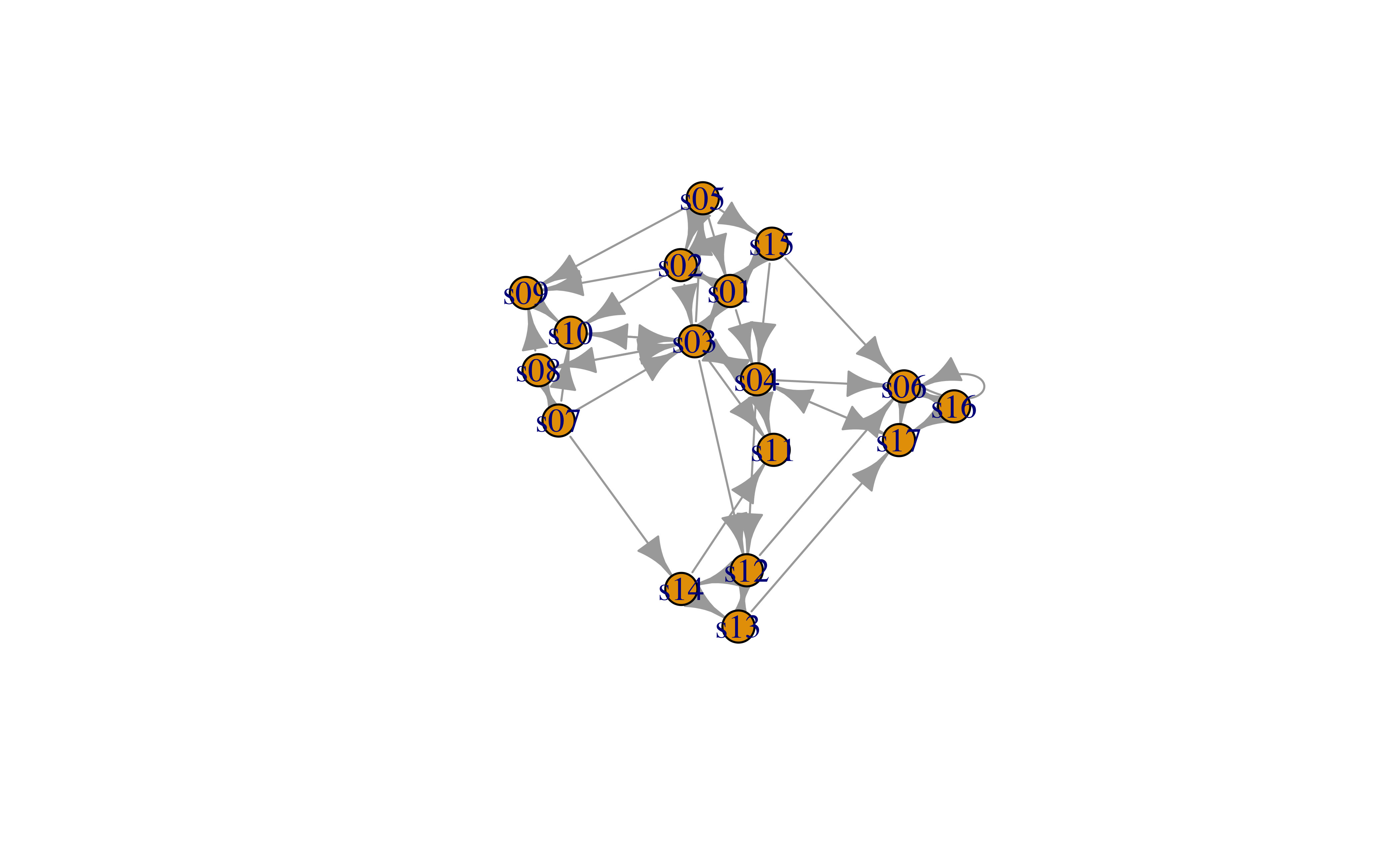

# Removing loops from the graph:
net <-
  igraph::simplify(net, remove.multiple = F, remove.loops = T)

# Let's and reduce the arrow size and remove the labels:
plot(net, edge.arrow.size = .4, vertex.label = NA)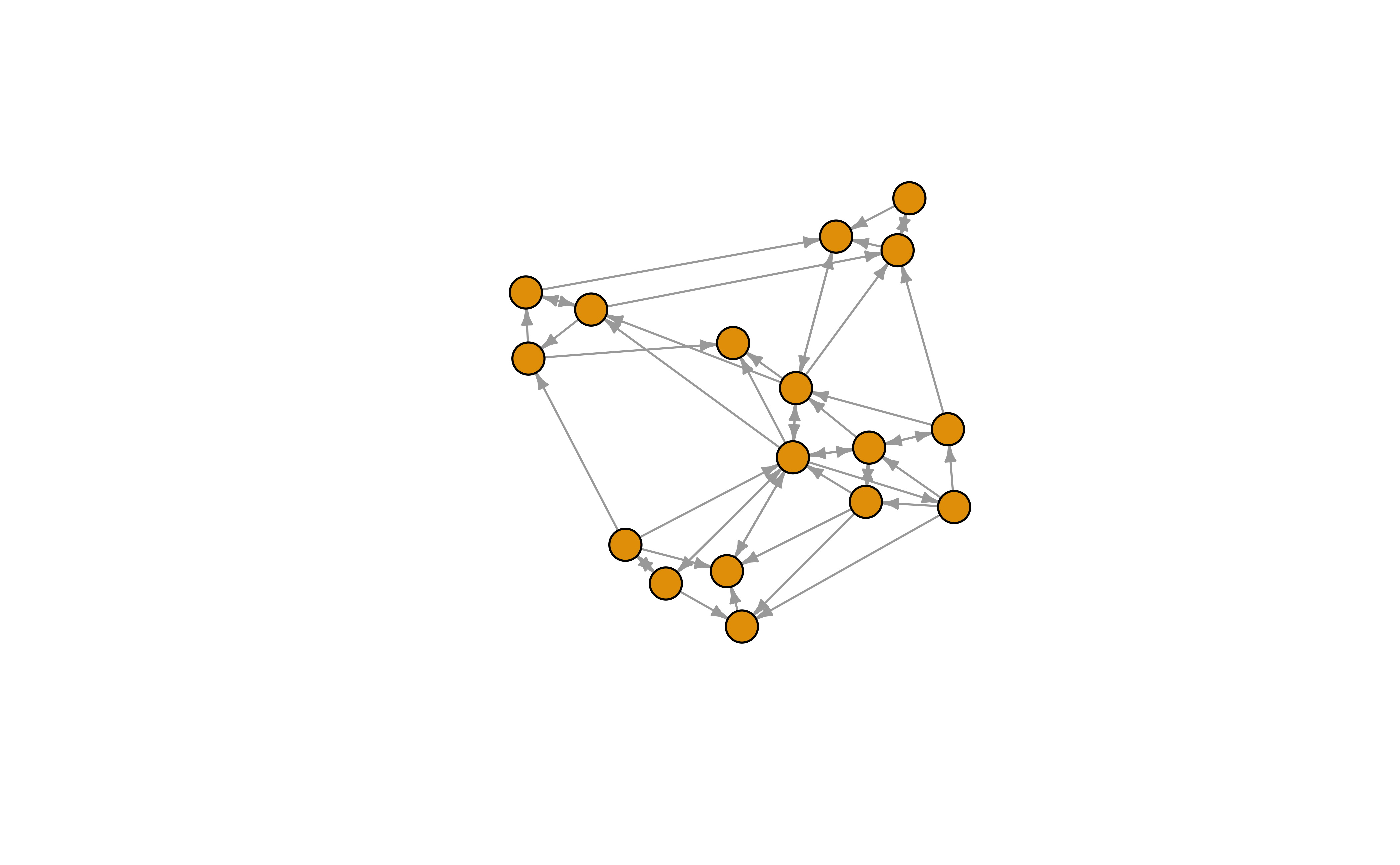

# Using tidygraph
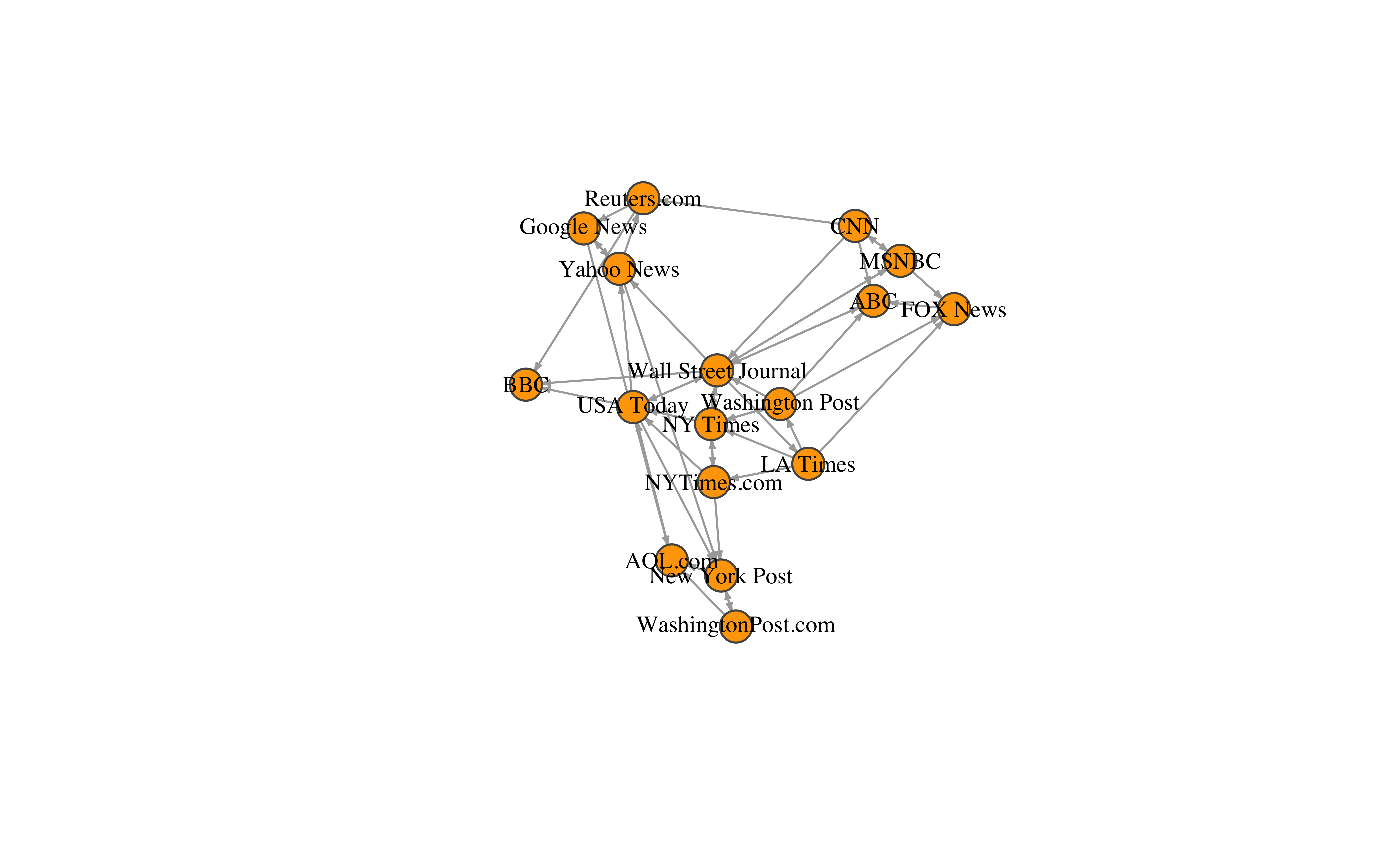
tbl_graph(nodes, links, directed = TRUE) %>%
  ggraph(., layout = "graphopt") +
  geom_edge_link(
    color = "grey",
    end_cap = circle(0.2, "cm"),
    start_cap = circle(0.2, "cm"),
    # clears an area near the node

    arrow = arrow(
      type = "closed",
      ends = "last",
      length = unit(3, "mm")
    )
  ) +
  geom_node_point(size = 8, shape = 21, fill = "orange") +
  geom_node_text(aes(label = id), size = 3)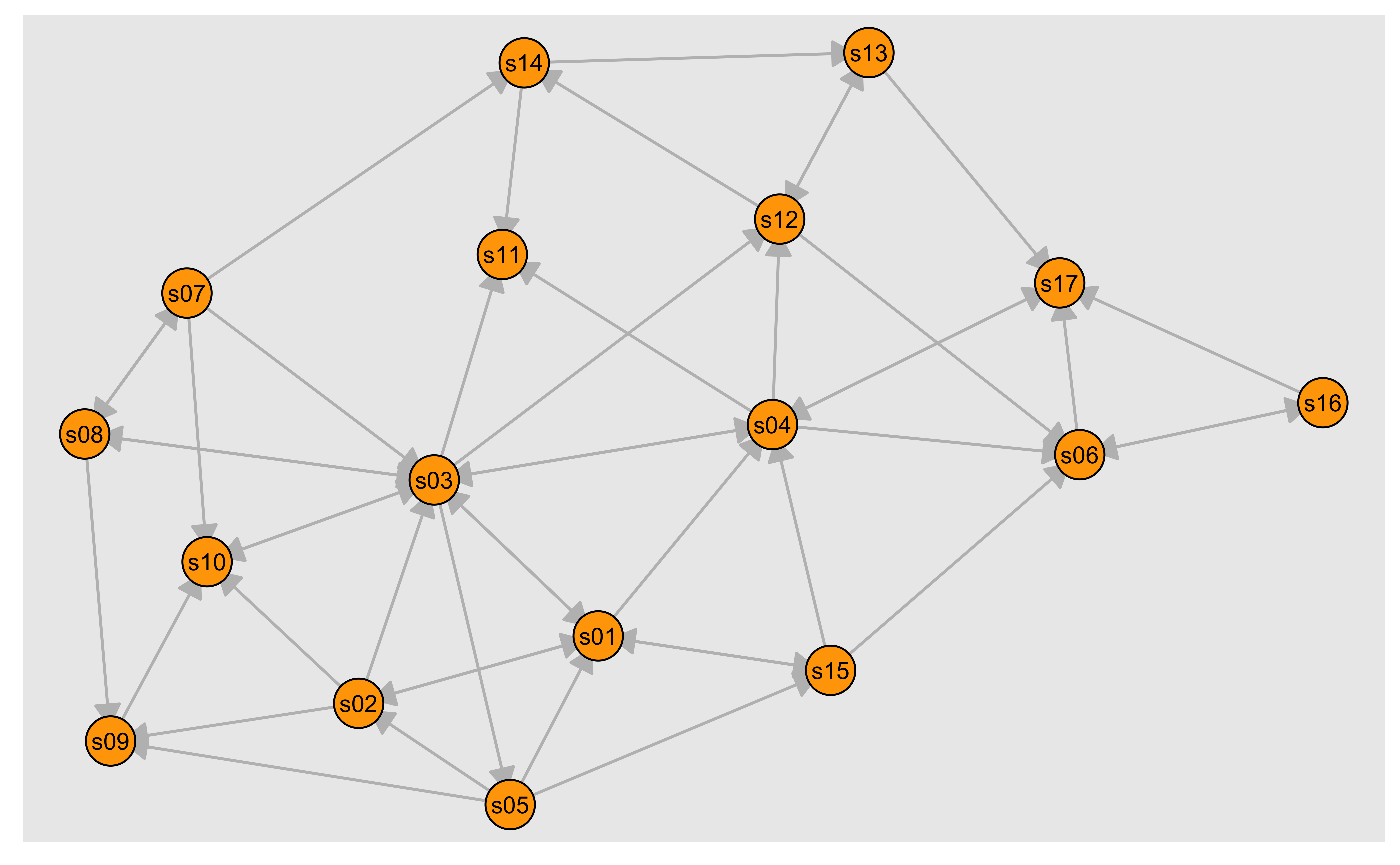

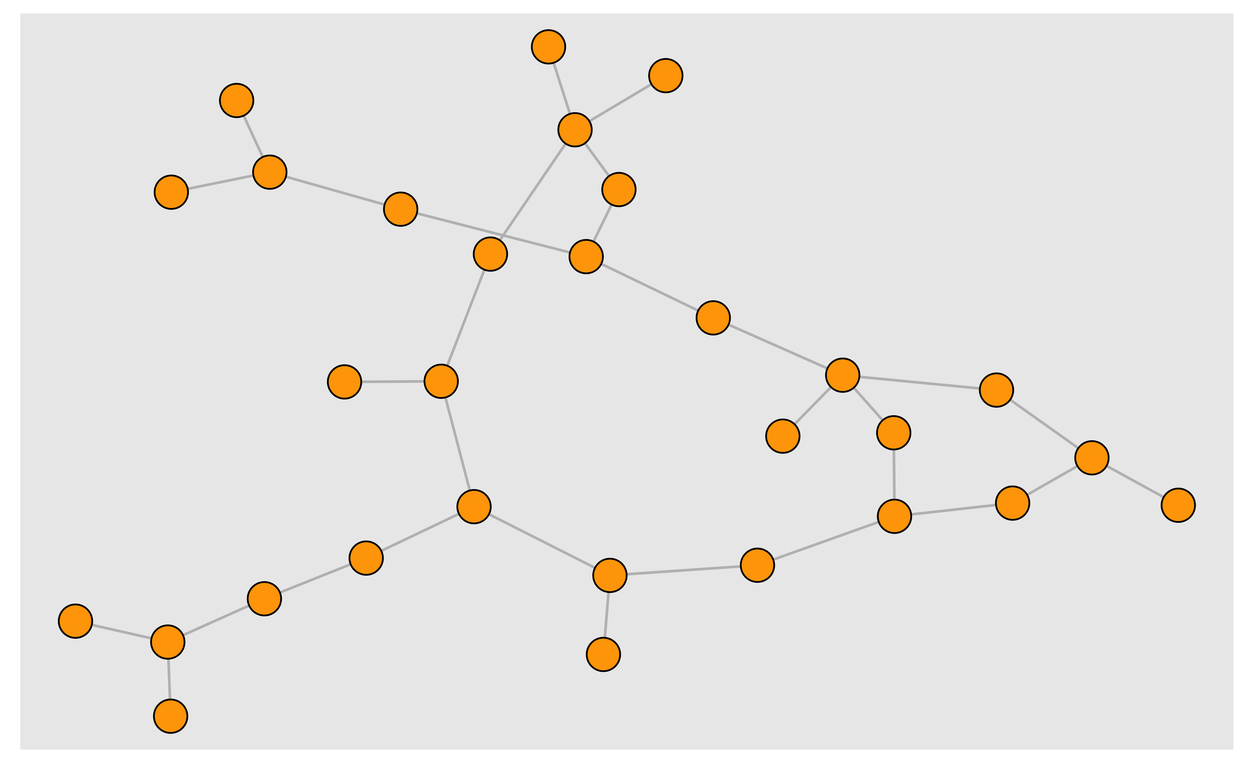
# Removing loops from the graph:
# From the docs:
# convert() is a shorthand for performing both `morph` and `crystallise` along with extracting a single tbl_graph (defaults to the first). For morphs w(h)ere you know they only create a single graph, and you want to keep it, this is an easy way.
#
tbl_graph(nodes, links, directed = TRUE) %>%
  convert(to_simple) %>%
  ggraph(., layout = "graphopt") +
  geom_edge_link(
    color = "grey",
    end_cap = circle(0.2, "cm"),
    start_cap = circle(0.2, "cm"),
    arrow = arrow(
      type = "closed",
      ends = "last",
      length = unit(3, "mm")
    )
  ) +
  geom_node_point(size = 6, shape = 21, fill = "orange")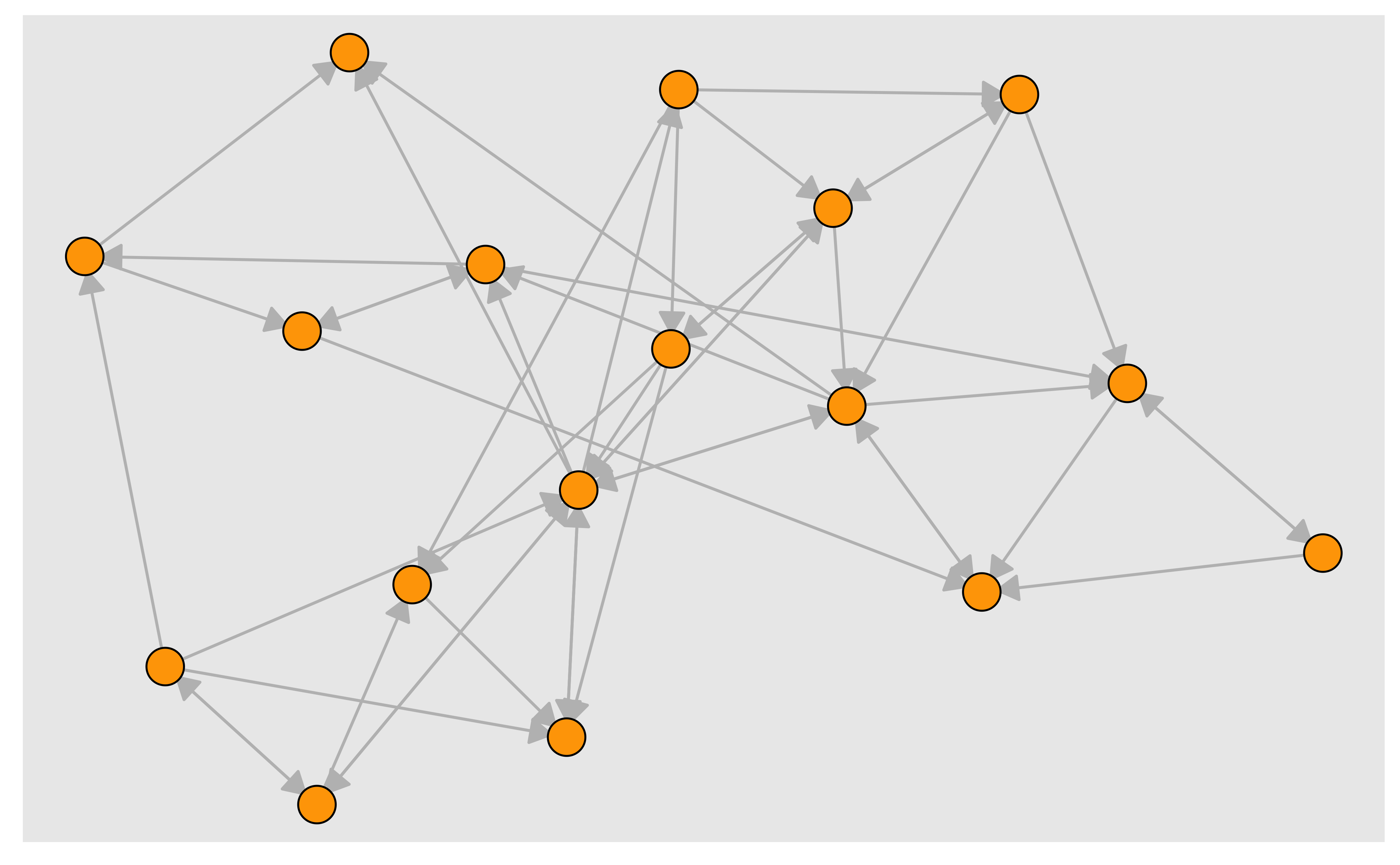

——-~~ DATASET 2: matrix ——–

# Read in the data:
nodes2 <- read.csv("./Dataset2-Media-User-Example-NODES.csv", header = T, as.is = T)
links2 <- read.csv("./Dataset2-Media-User-Example-EDGES.csv", header = T, row.names = 1)

# Examine the data:
head(nodes2)

ABCDEFGHIJ0123456789

	id <chr>	media <chr>	media.type <int>	media.name <chr>	audience.size <int>
1	s01	NYT	1	Newspaper	20
2	s02	WaPo	1	Newspaper	25
3	s03	WSJ	1	Newspaper	30
4	s04	USAT	1	Newspaper	32
5	s05	LATimes	1	Newspaper	20
6	s06	CNN	2	TV	56

head(links2)

ABCDEFGHIJ0123456789

	U01 <int>	U02 <int>	U03 <int>	U04 <int>	U05 <int>	U06 <int>	U07 <int>	U08 <int>	U09 <int>
s01	1	1	1	0	0	0	0	0	0
s02	0	0	0	1	1	0	0	0	0
s03	0	0	0	0	0	1	1	1	1
s04	0	0	0	0	0	0	0	0	1
s05	0	0	0	0	0	0	0	0	0
s06	0	0	0	0	0	0	0	0	0

# links2 is a matrix for a two-mode network:
links2 <- as.matrix(links2)
dim(links2)

[1] 10 20

dim(nodes2)

[1] 30  5

Note: What is a two-mode network? A network that as a node$type variable and can be a bipartite or a k-partite network as a result.

# Create an igraph network object from the two-mode matrix:
net2 <- igraph::graph_from_incidence_matrix(links2)

# To transform a one-mode network matrix into an igraph object,
# we would use graph_from_adjacency_matrix()

# A built-in vertex attribute 'type' shows which mode vertices belong to.
table(V(net2)$type)


FALSE  TRUE 
   10    20

# Basic igraph plot
plot(net2, vertex.label = NA)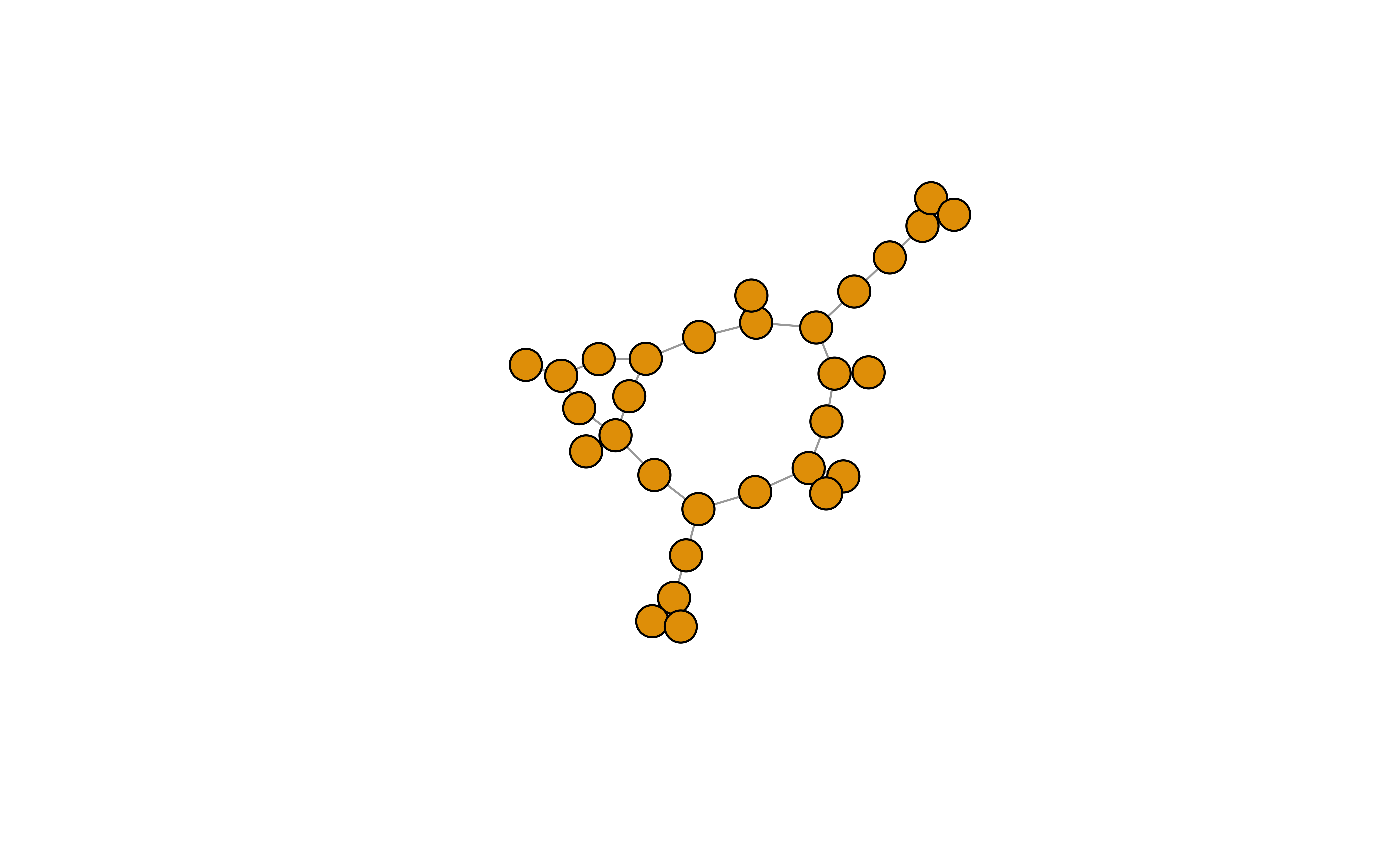

# using tidygraph
# For all objects that are not node and edge data_frames
# tidygraph uses `as_tbl_graph()`
#
graph <- as_tbl_graph(links2)
graph %>%
  activate(nodes) %>%
  as_tibble()

ABCDEFGHIJ0123456789

type <lgl>	name <chr>
FALSE	s01
FALSE	s02
FALSE	s03
FALSE	s04
FALSE	s05
FALSE	s06
FALSE	s07
FALSE	s08
FALSE	s09
FALSE	s10

graph %>%
  activate(edges) %>%
  as_tibble()

ABCDEFGHIJ0123456789

from <int>	to <int>	weight <dbl>
1	11	1
1	12	1
1	13	1
2	14	1
2	15	1
2	30	1
3	16	1
3	17	1
3	18	1
3	19	1

graph %>%
  ggraph(., layout = "graphopt") +
  geom_edge_link(color = "grey") +
  geom_node_point(
    fill = "orange",
    shape = 21, size = 6,
    color = "black"
  )

# Examine the resulting object:
class(net2)

[1] "igraph"

net2

IGRAPH 330c2c6 UN-B 30 31 -- 
+ attr: type (v/l), name (v/c)
+ edges from 330c2c6 (vertex names):
 [1] s01--U01 s01--U02 s01--U03 s02--U04 s02--U05 s02--U20 s03--U06 s03--U07
 [9] s03--U08 s03--U09 s04--U09 s04--U10 s04--U11 s05--U11 s05--U12 s05--U13
[17] s06--U13 s06--U14 s06--U17 s07--U14 s07--U15 s07--U16 s08--U16 s08--U17
[25] s08--U18 s08--U19 s09--U06 s09--U19 s09--U20 s10--U01 s10--U11

Note: The remaining attributes for the nodes ( in data frame nodes2) are not (yet) a part of the graph, either with igraph or with tidygraph.

3. Network plots in ‘igraph’

——~~ Plot parameters in igraph ——–

Check out the node options (starting with ‘vertex.’) and the edge options (starting with ‘edge.’).

Type ?igraph.plotting in your console

?igraph.plotting

We can set the node & edge options in two ways - one is to specify them in the plot() function, as we are doing below.

Plot with curved edges (edge.curved = .1) and reduce arrow size:

plot(net, edge.arrow.size = .4, edge.curved = .1)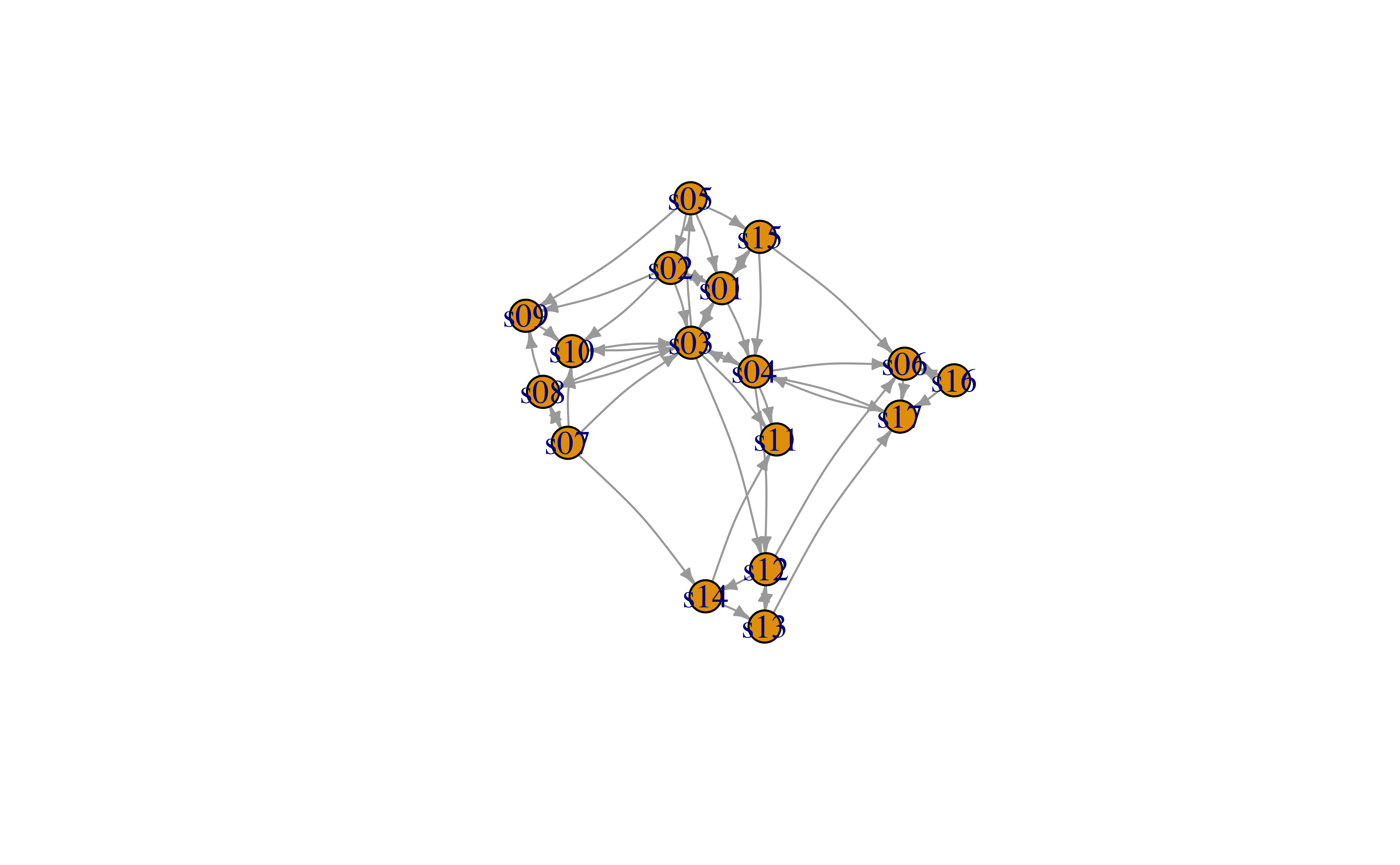

# Using tidygraph
graph <- tbl_graph(nodes, links, directed = TRUE)
graph

# A tbl_graph: 17 nodes and 49 edges
#
# A directed multigraph with 1 component
#
# Node Data: 17 × 5 (active)
   id    media               media.type type.label audience.size
   <chr> <chr>                    <int> <chr>              <int>
 1 s01   NY Times                     1 Newspaper             20
 2 s02   Washington Post              1 Newspaper             25
 3 s03   Wall Street Journal          1 Newspaper             30
 4 s04   USA Today                    1 Newspaper             32
 5 s05   LA Times                     1 Newspaper             20
 6 s06   New York Post                1 Newspaper             50
 7 s07   CNN                          2 TV                    56
 8 s08   MSNBC                        2 TV                    34
 9 s09   FOX News                     2 TV                    60
10 s10   ABC                          2 TV                    23
11 s11   BBC                          2 TV                    34
12 s12   Yahoo News                   3 Online                33
13 s13   Google News                  3 Online                23
14 s14   Reuters.com                  3 Online                12
15 s15   NYTimes.com                  3 Online                24
16 s16   WashingtonPost.com           3 Online                28
17 s17   AOL.com                      3 Online                33
#
# Edge Data: 49 × 4
   from    to type      weight
  <int> <int> <chr>      <int>
1     1     2 hyperlink     22
2     1     3 hyperlink     22
3     1     4 hyperlink     21
# ℹ 46 more rows

graph %>% ggraph(., layout = "graphopt") +
  geom_edge_arc(
    color = "grey",
    strength = 0.1,
    end_cap = circle(.2, "cm"),
    arrow = arrow(
      type = "closed",
      ends = "both",
      length = unit(3, "mm")
    )
  ) +
  geom_node_point(
    fill = "orange",
    shape = 21,
    size = 8,
    color = "black"
  ) +
  geom_node_text(aes(label = id), size = 3)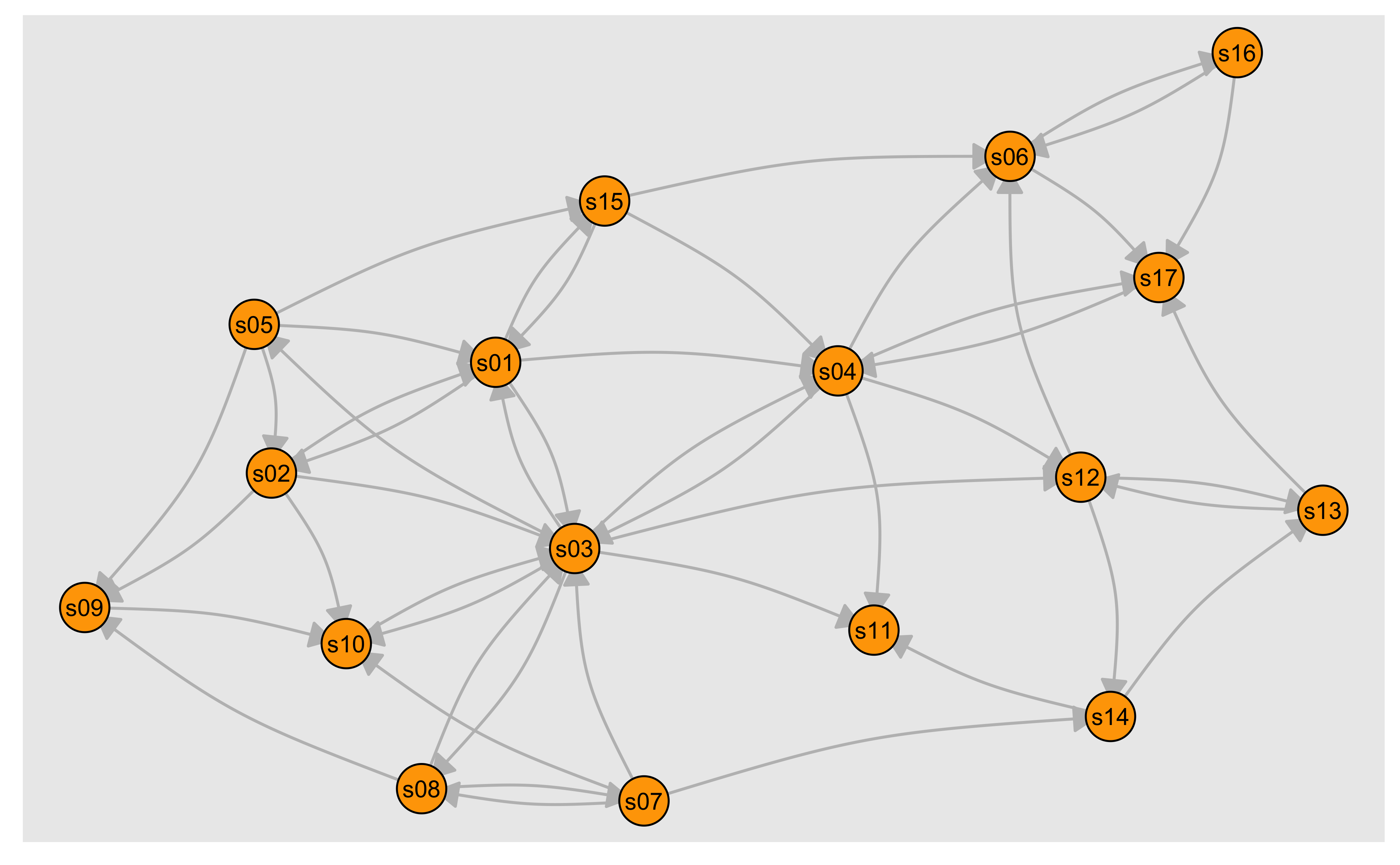

Set node color to orange and the border color to hex 555555
Replace the vertex label with the node names stored in “media”

plot(
  net,
  edge.arrow.size = .2,
  edge.curved = 0,
  vertex.color = "orange",
  vertex.frame.color = "#555555",
  vertex.label = V(net)$media,
  vertex.label.color = "black",
  vertex.label.cex = .7
)

# Using tidygraph
# graph <- tbl_graph(nodes, links, directed = TRUE)
# graph
graph %>%
  ggraph(., layout = "gem") +
  geom_edge_link(
    color = "grey",
    end_cap = circle(.3, "cm"),
    arrow = arrow(
      type = "closed",
      ends = "both",
      length = unit(1, "mm")
    )
  ) +
  geom_node_point(
    fill = "orange",
    shape = 21,
    size = 6,
    color = "#555555"
  ) +
  geom_node_text(aes(label = media))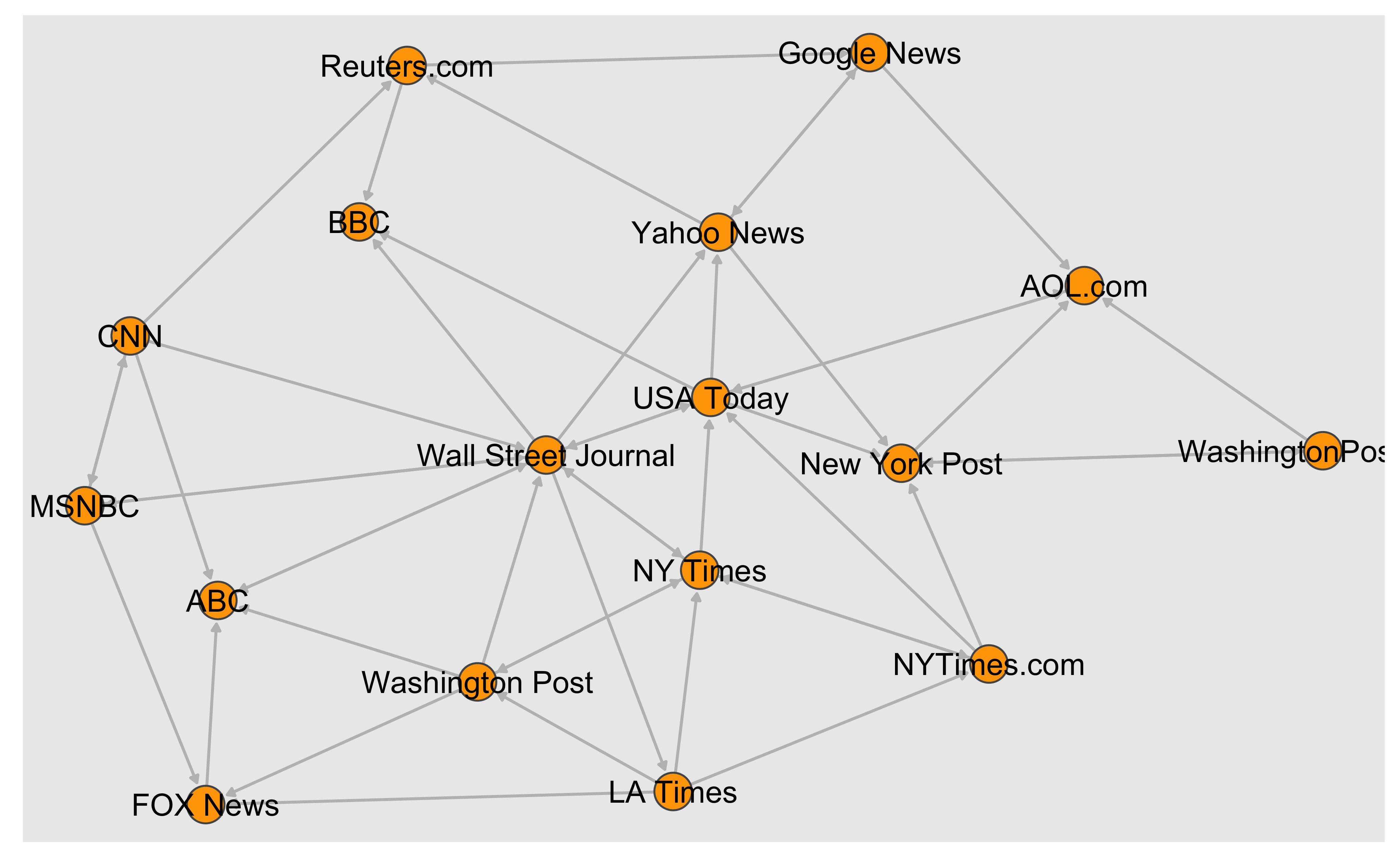

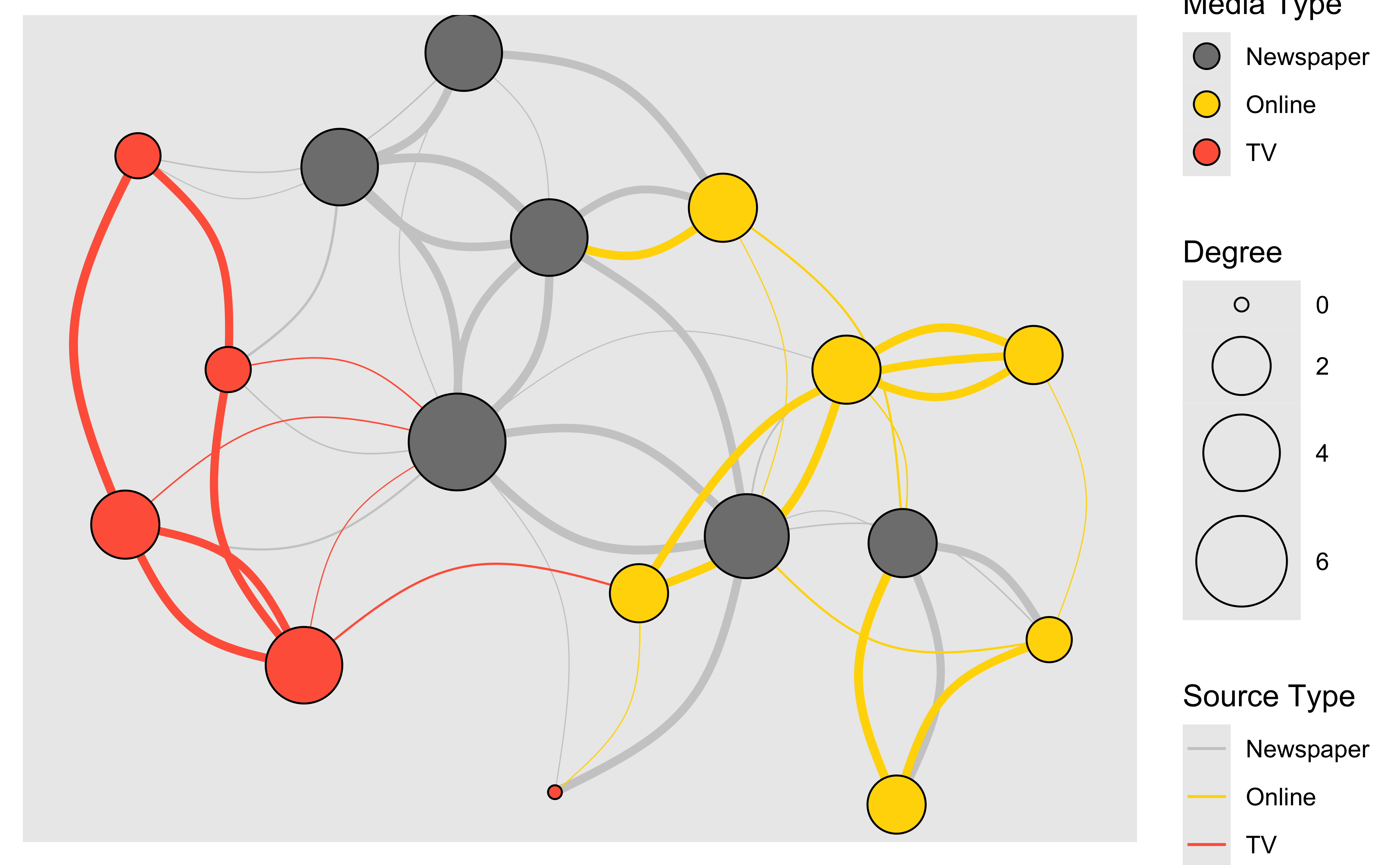
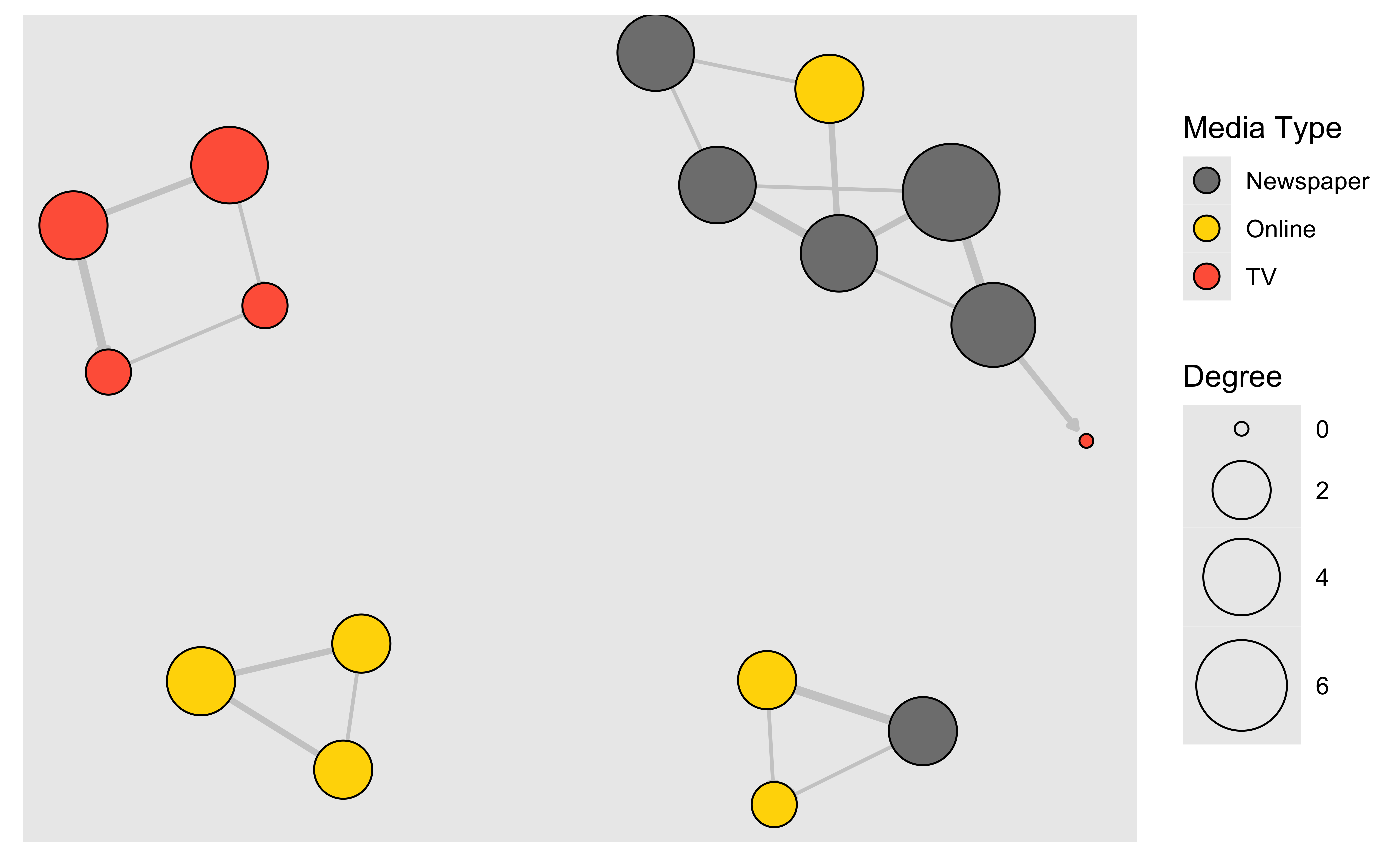
The second way to set attributes is to add them to the igraph object.

Generate colors based on media type:

colrs <- c("gray50", "tomato", "gold")
V(net)$color <- colrs[V(net)$media.type]
plot(net)

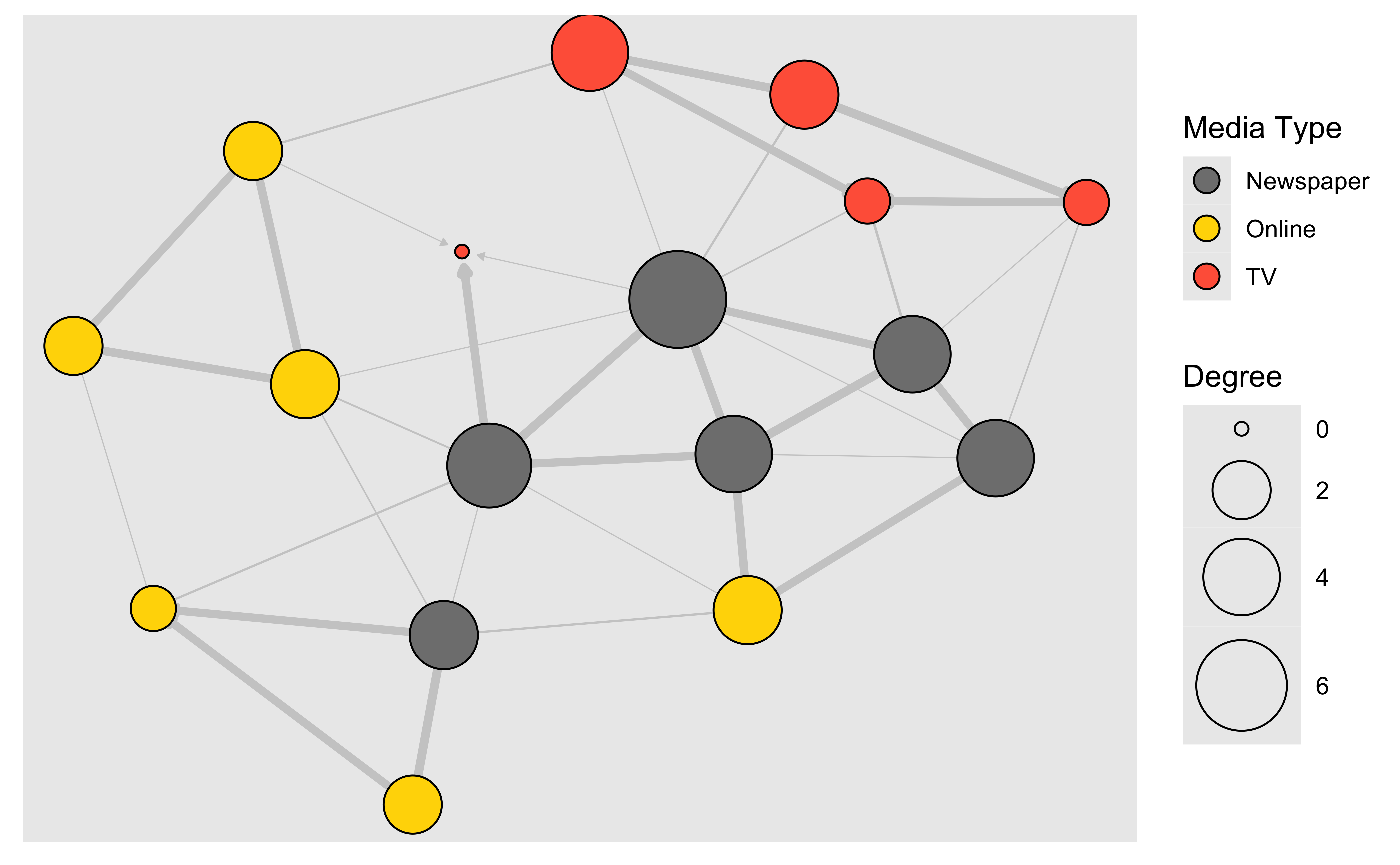
Compute node degrees (#links) and use that to set node size:

deg <- igraph::degree(net, mode = "all")
V(net)$size <- deg * 3
# Alternatively, we can set node size based on audience size:
V(net)$size <- V(net)$audience.size * 0.7
V(net)$size

 [1] 14.0 17.5 21.0 22.4 14.0 35.0 39.2 23.8 42.0 16.1 23.8 23.1 16.1  8.4 16.8
[16] 19.6 23.1

# The labels are currently node IDs.
# Setting them to NA will render no labels:
V(net)$label.color <- "black"
V(net)$label <- NA

# Set edge width based on weight:
E(net)$width <- E(net)$weight / 6

# change arrow size and edge color:
E(net)$arrow.size <- .2
E(net)$edge.color <- "gray80"

# We can even set the network layout:
graph_attr(net, "layout") <- layout_with_lgl
plot(net)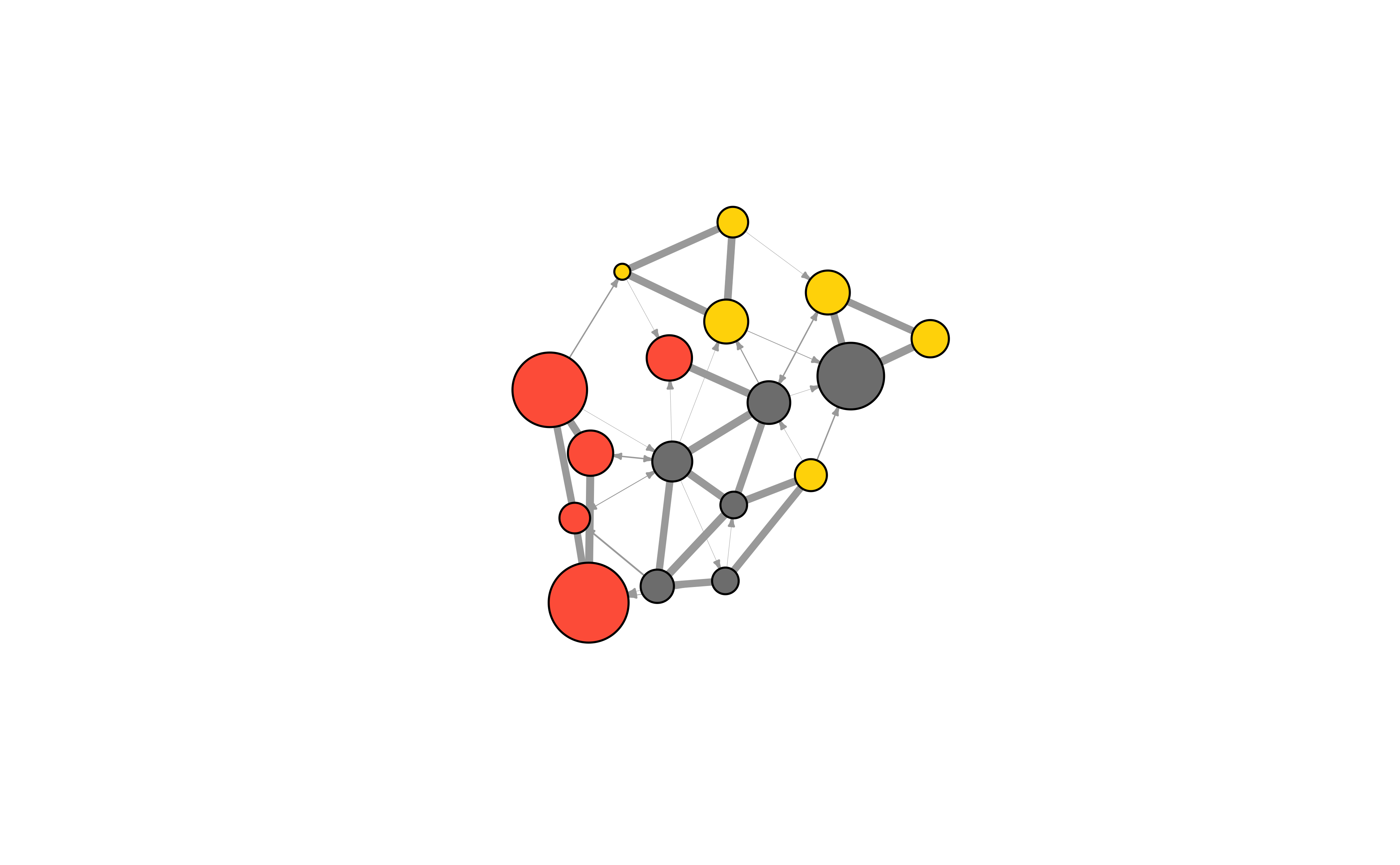

# Using tidygraph
# graph <- tbl_graph(nodes, links, directed = TRUE)
# graph
graph %>%
  activate(nodes) %>%
  mutate(size = centrality_degree()) %>%
  ggraph(., layout = "lgl") +
  geom_edge_link(
    aes(width = weight),
    color = "grey80",
    end_cap = circle(.2, "cm"),
    arrow = arrow(
      type = "closed",
      ends = "last",
      length = unit(1, "mm")
    )
  ) +
  geom_node_point(aes(fill = type.label, size = size),
    shape = 21,
    color = "black"
  ) +
  scale_fill_manual(
    name = "Media Type",
    values = c("grey50", "gold", "tomato")
  ) +
  scale_edge_width(range = c(0.2, 1.5), guide = "none") +
  scale_size_continuous("Degree", range = c(2, 16)) +

  guides(fill = guide_legend(
    title = "Media Type",
    override.aes = list(pch = 21, size = 4)
  ))

We can also override the attributes explicitly in the plot:

plot(net, edge.color = "orange", vertex.color = "gray50")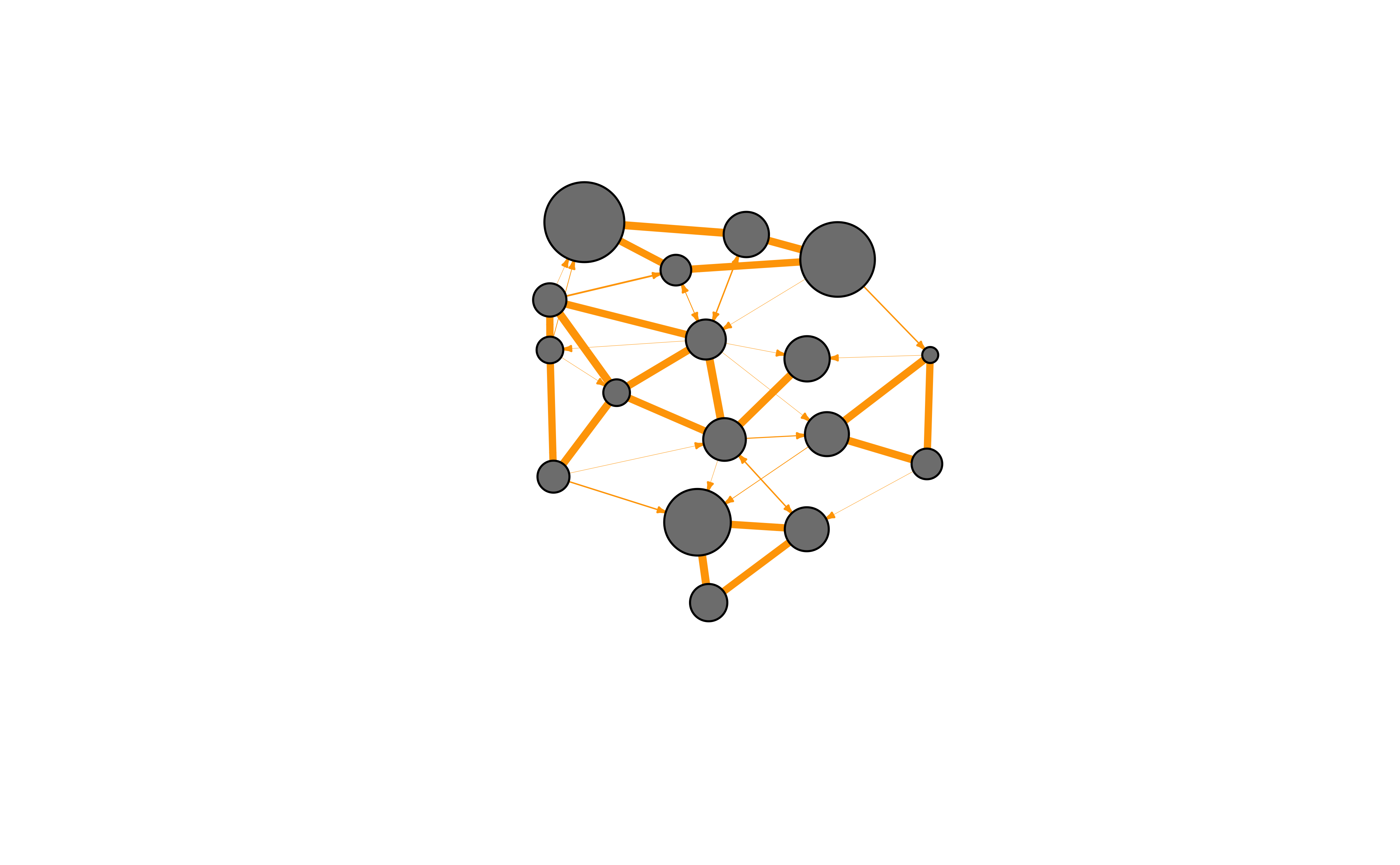

We can also add a legend explaining the meaning of the colors we used:

plot(net)
legend(
  x = -2.1, y = -1.1,
  c("Newspaper", "Television", "Online News"),
  pch = 21, col = "#777777",
  pt.bg = colrs, pt.cex = 2.5, bty = "n", ncol = 1
)

# legends are automatic with the tidygraph + ggraph flow

Sometimes, especially with semantic networks, we may be interested in plotting only the labels of the nodes:

plot(net,
  vertex.shape = "none", vertex.label = V(net)$media,
  vertex.label.font = 2, vertex.label.color = "gray40",
  vertex.label.cex = .7, edge.color = "gray85"
)

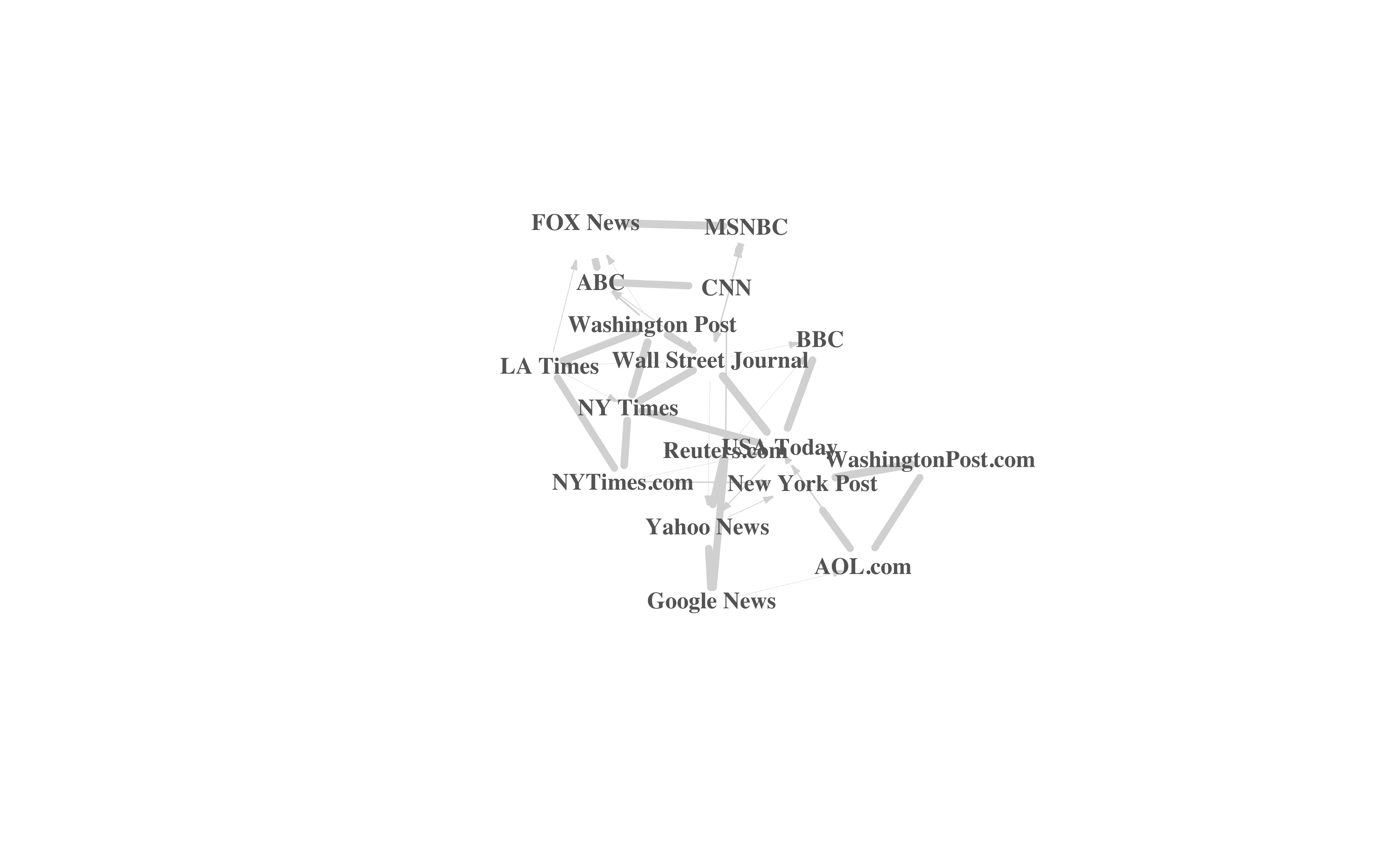
# using tidygraph

ggraph(net, layout = "gem") +
  geom_edge_link(
    color = "grey80", width = 2,
    end_cap = circle(0.5, "cm"),
    start_cap = circle(0.5, "cm")
  ) +
  geom_node_text(aes(label = media))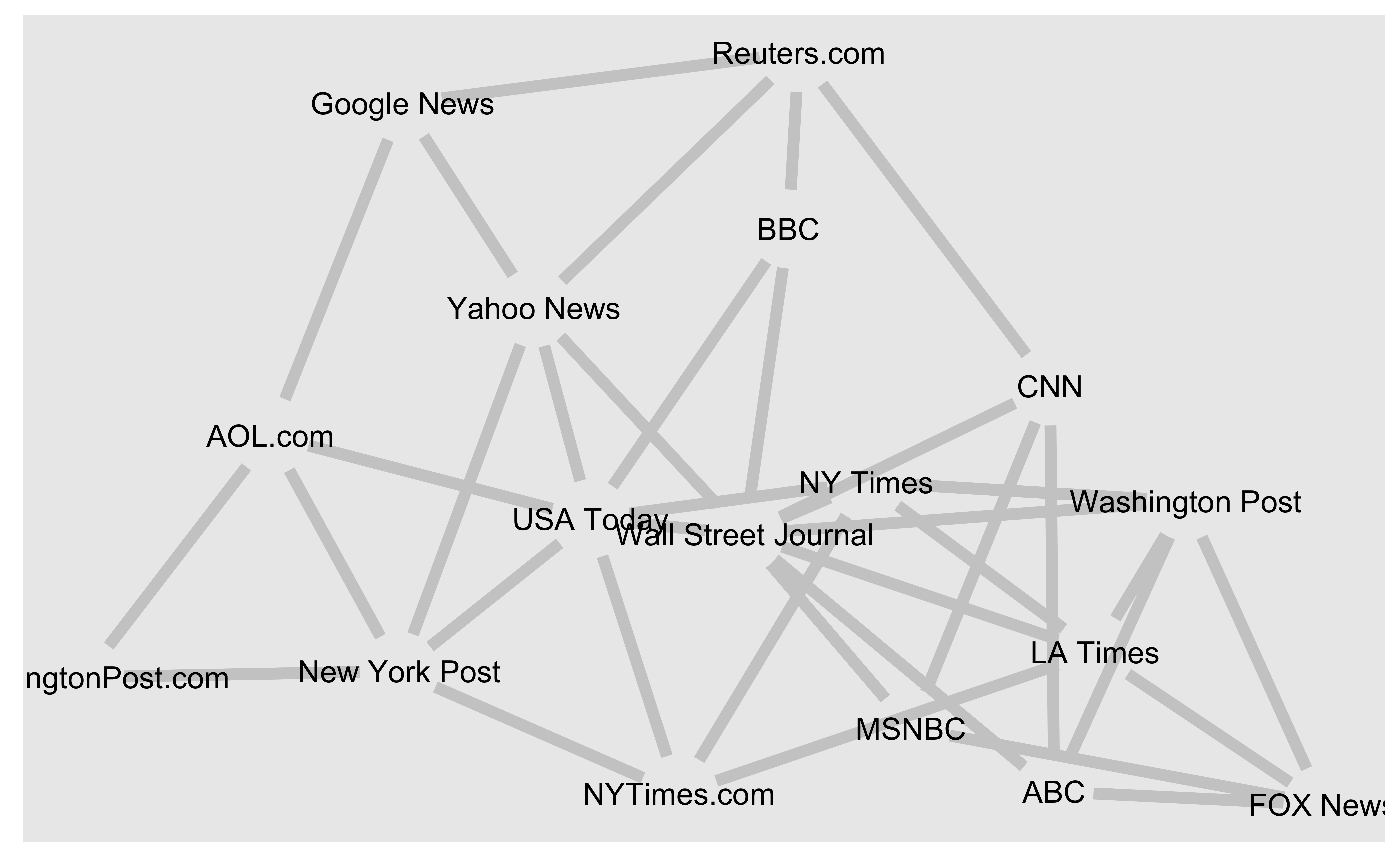

Let’s color the edges of the graph based on their source node color. We’ll get the starting node for each edge with ends().

Note: Edge attribute is being set by start node.

edge.start <- ends(net, es = E(net), names = F)[, 1]
edge.col <- V(net)$color[edge.start] # How simple this is !!!
# The three colors are recycled
#
plot(net, edge.color = edge.col, edge.curved = .4)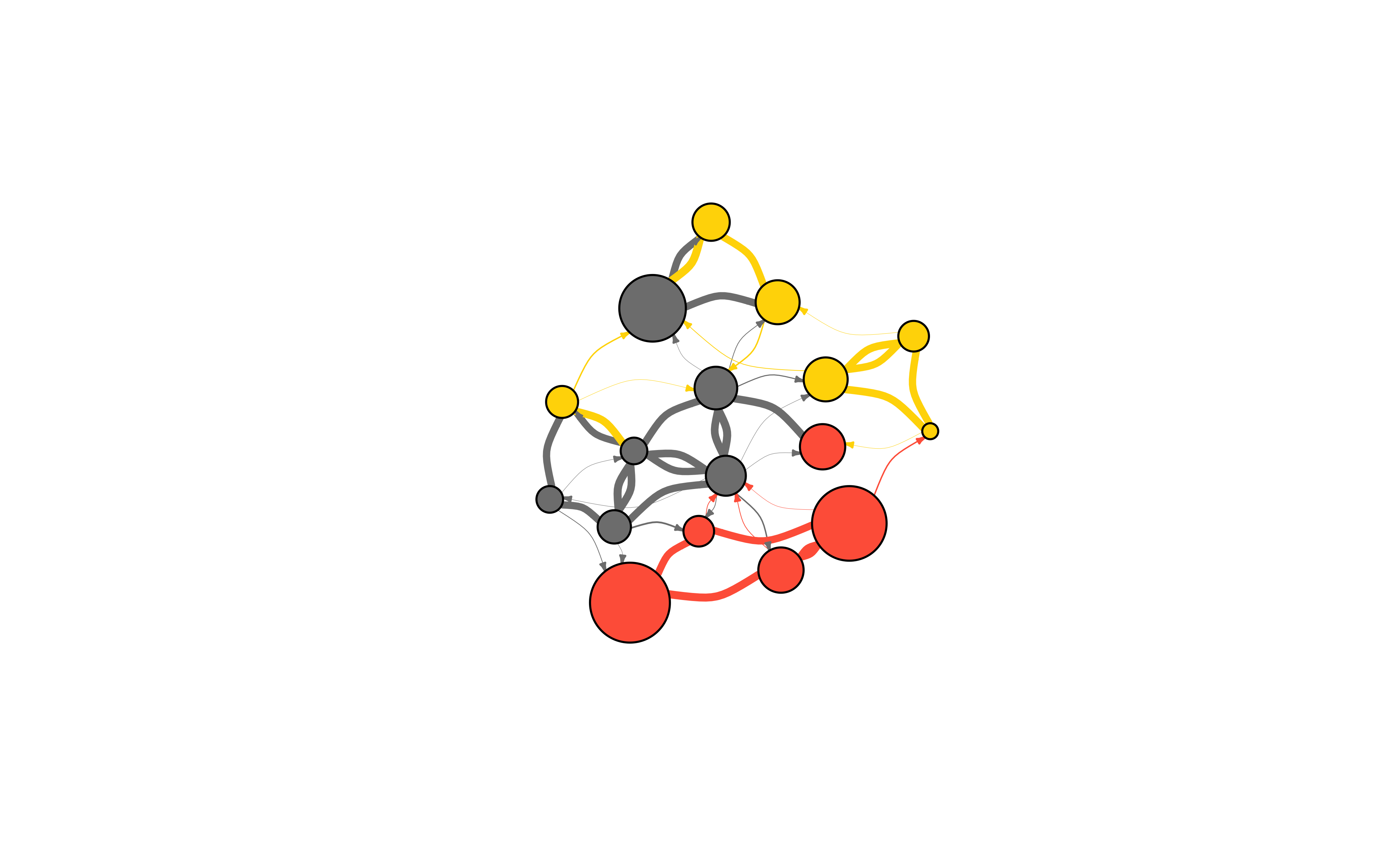

NOTE: The source node colour has been set using the media.type, which is a node attribute. Node attributes are not typically accessible to edges. So we need to build a combo data frame using dplyr, so that edges can use this node attribute. ( There may be other ways…)

# Using tidygraph
# Make a "combo" data frame of nodes *and* edges with left_join()
# Join by `from` so that type.label is based on from = edge.start

links %>%
  left_join(., nodes, by = c("from" = "id")) %>%
  tbl_graph(edges = ., nodes = nodes) %>%
  mutate(size = centrality_degree()) %>%
  ggraph(., layout = "lgl") +
  geom_edge_arc(
    aes(
      color = type.label,
      width = weight
    ),
    strength = 0.3
  ) +
  geom_node_point(
    aes(
      fill = type.label,
      # type.label is now available as edge attribute
      size = size
    ),
    shape = 21,
    color = "black"
  ) +
  scale_fill_manual(
    name = "Media Type",
    values = c("grey50", "gold", "tomato"),
    guide = "legend"
  ) +
  scale_edge_color_manual(
    name = "Source Type",
    values = c("grey80", "gold", "tomato")
  ) +
  scale_edge_width(range = c(0.2, 1.5), guide = "none") +
  scale_size_continuous("Degree", range = c(2, 16)) +
  # not "limits"!
  guides(fill = guide_legend(override.aes = list(
    pch = 21,
    size = 4
  )))

——-~~ Network Layouts in ‘igraph’ ——–

Network layouts are algorithms that return coordinates for each node in a network.

Let’s generate a slightly larger 100-node graph using a preferential attachment model (Barabasi-Albert).

net.bg <- sample_pa(n = 100, power = 1.2)
V(net.bg)$size <- 8
V(net.bg)$frame.color <- "white"
V(net.bg)$color <- "orange"
V(net.bg)$label <- ""
E(net.bg)$arrow.mode <- 0
plot(net.bg)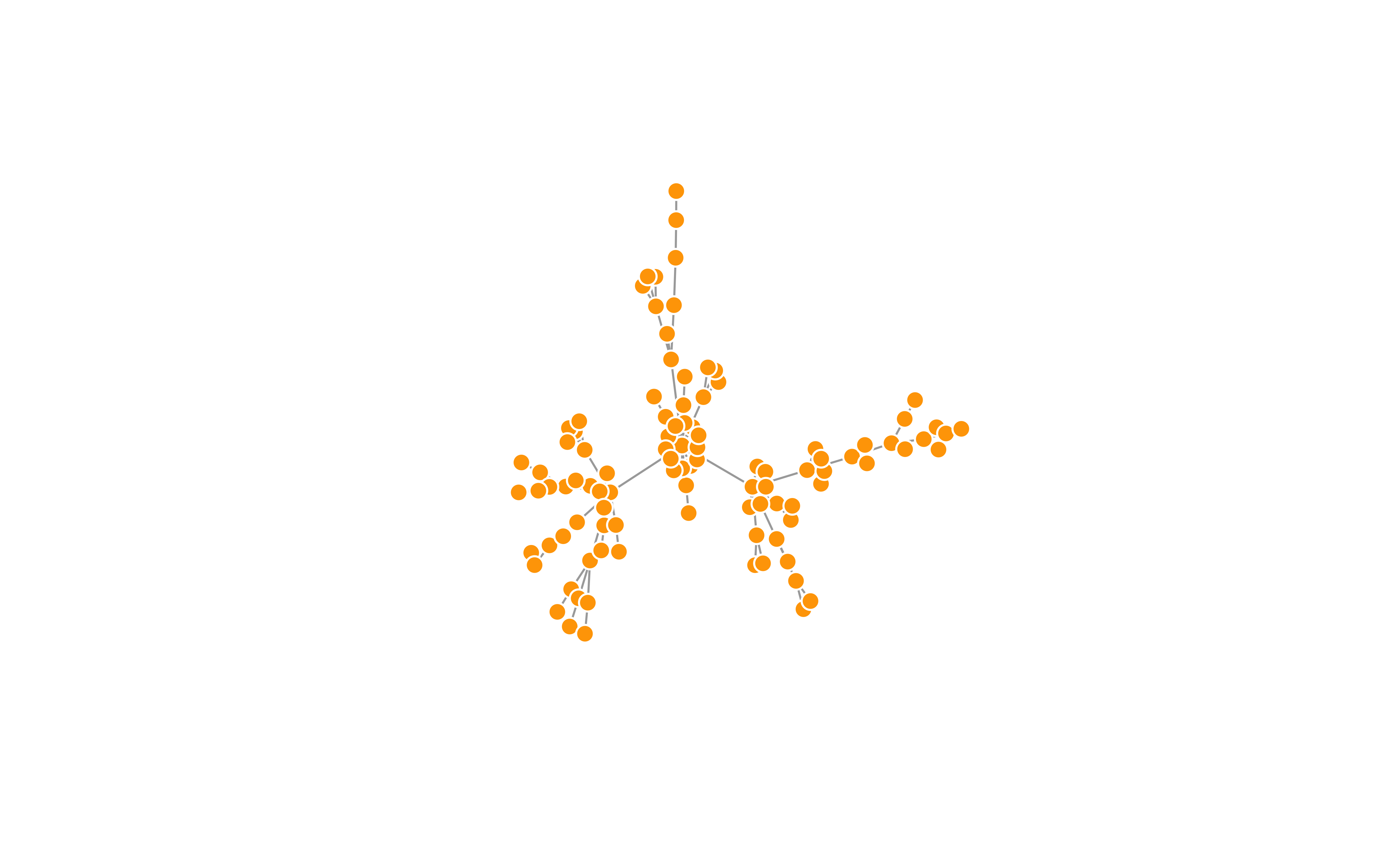

# Using tidygraph
graph <- play_barabasi_albert(n = 100, power = 1.2)
graph %>%
  ggraph(., layout = "graphopt") +
  geom_edge_link(color = "grey") +
  geom_node_point(color = "orange", size = 4) +
  theme_graph()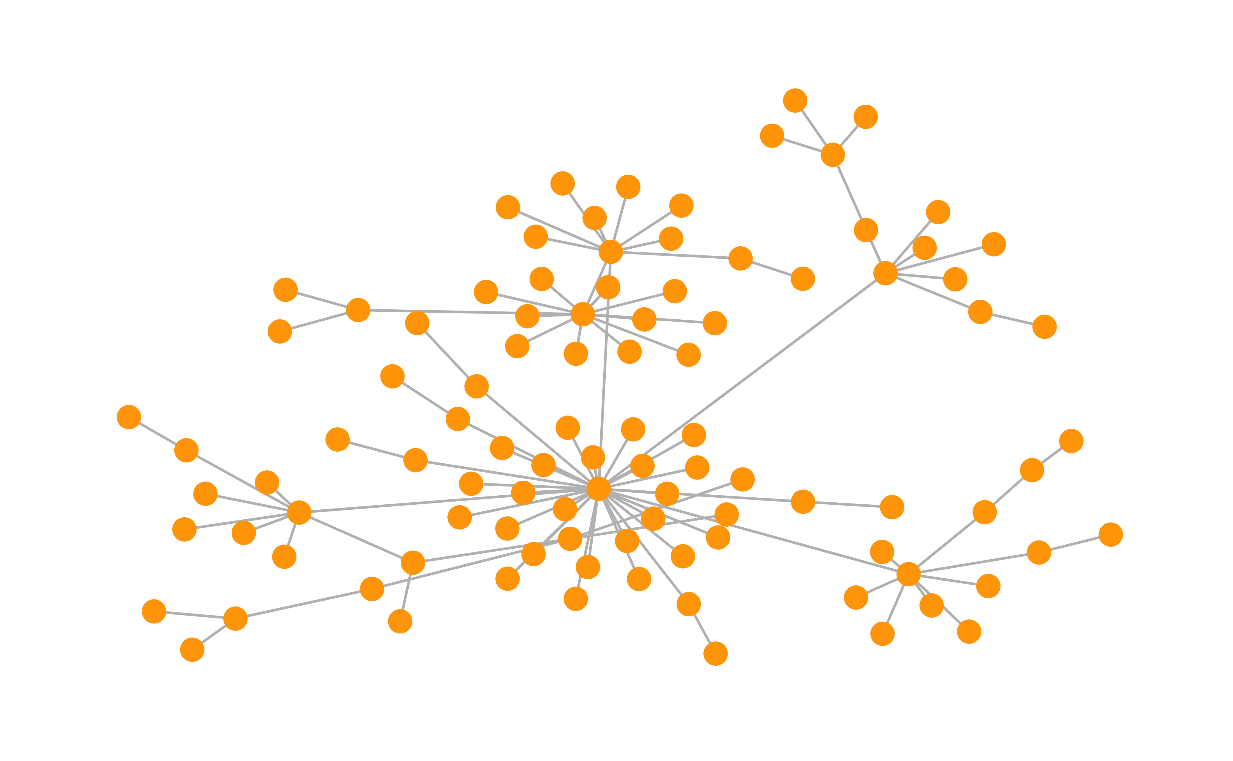

Now let’s plot this network using the layouts available in igraph. You can set the layout in the plot function:

plot(net.bg, layout = layout_randomly)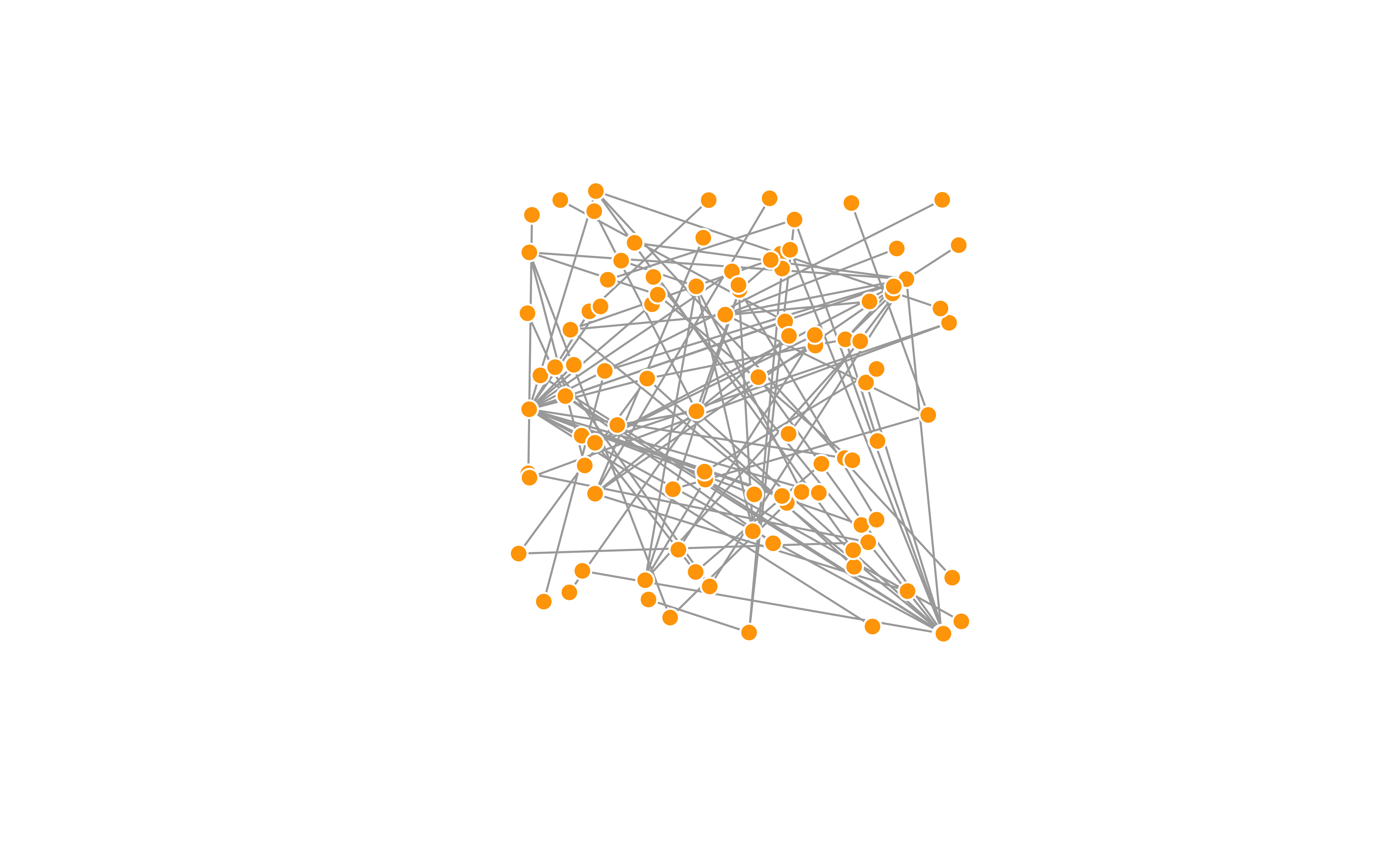

Or calculate the vertex coordinates in advance:

l <- layout_in_circle(net.bg)
plot(net.bg, layout = l)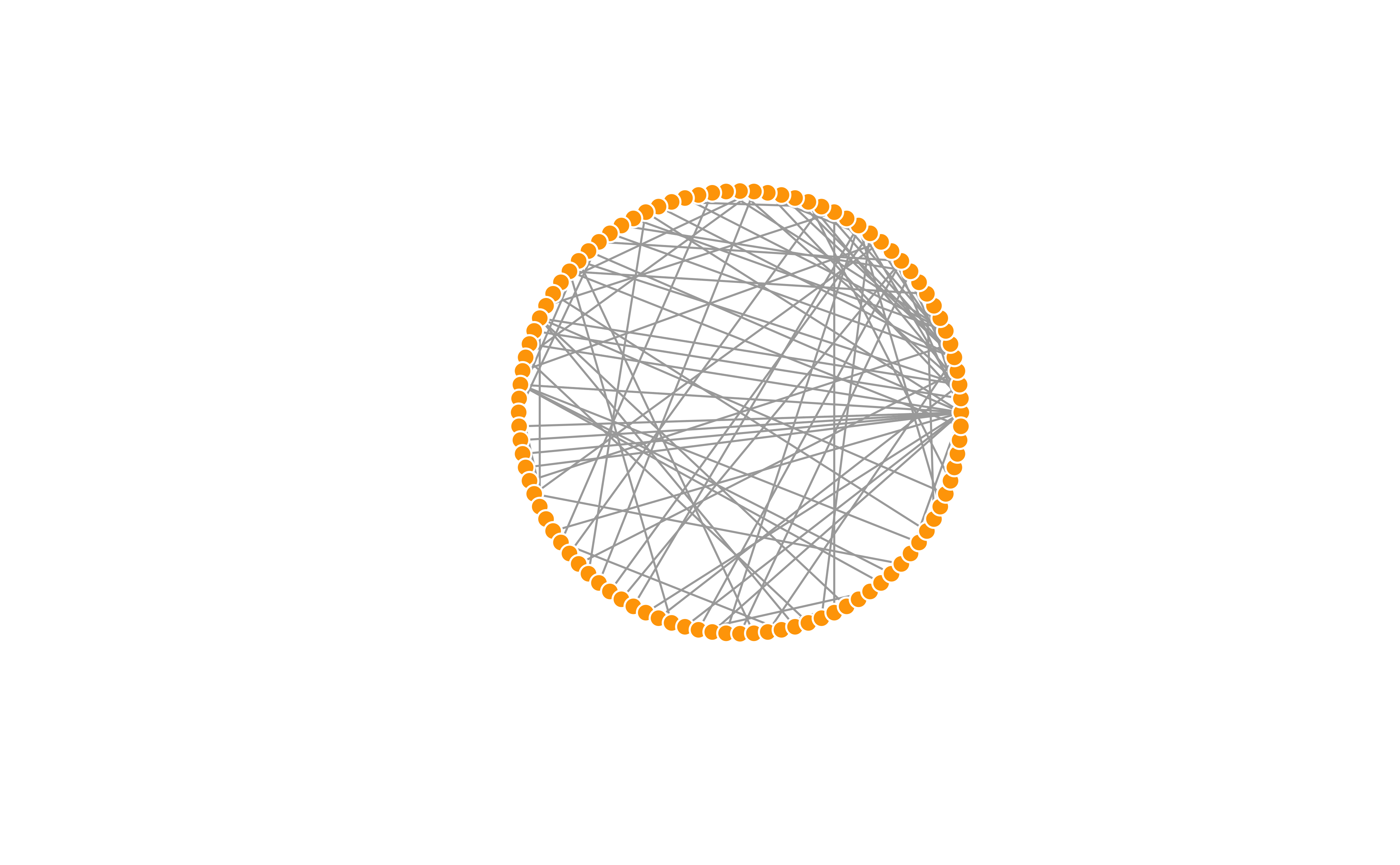

# Using tidygraph
# graph <- play_barabasi_albert(n = 100, power = 1.2)
graph %>% ggraph(., layout = "circle") +
  geom_edge_link(color = "grey") +
  geom_node_point(color = "orange", size = 2) +
  theme_graph() +
  theme(aspect.ratio = 1)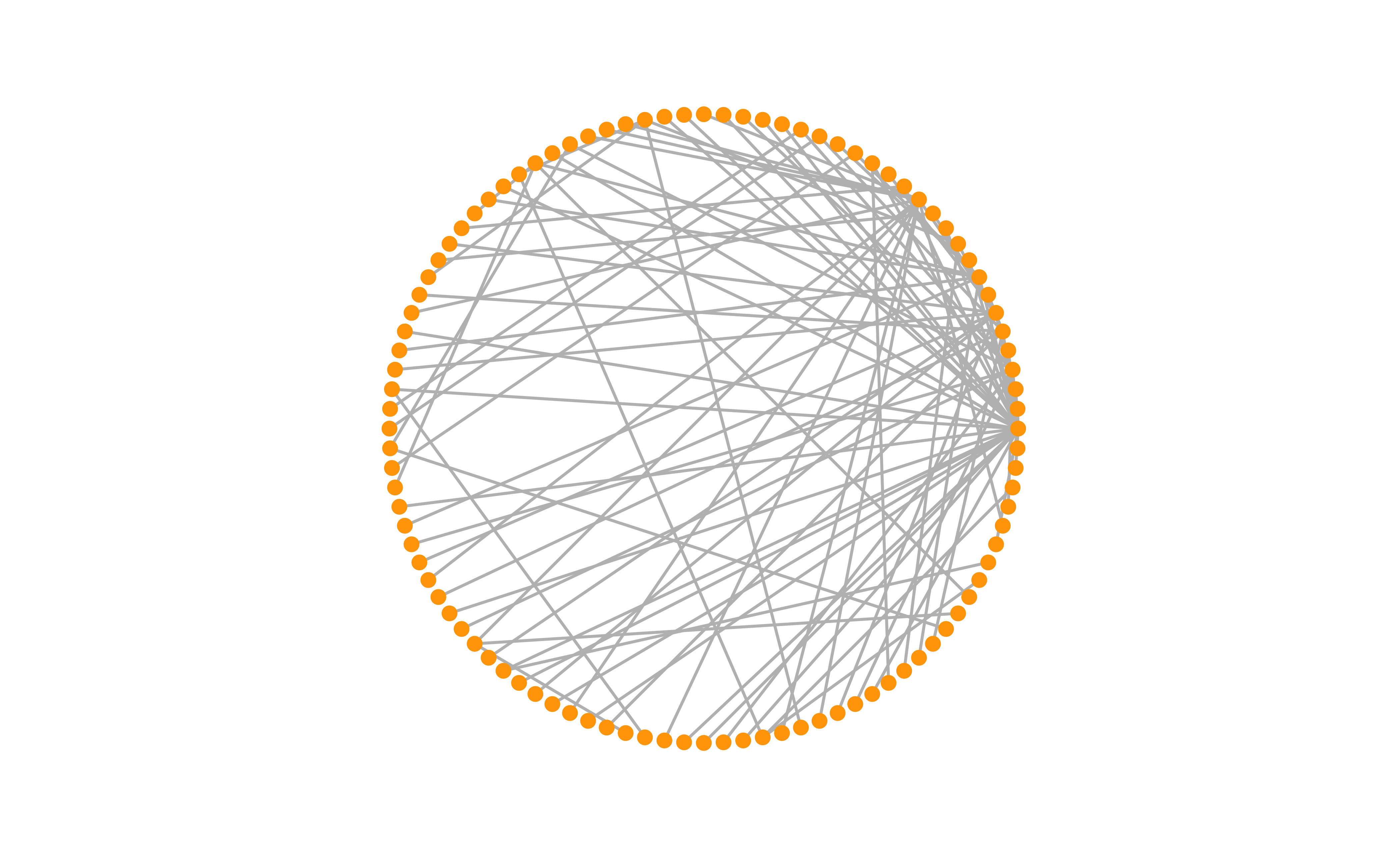

l is simply a matrix of x,y coordinates (N x 2) for the N nodes in the graph. You can generate your own:

l <- cbind(1:vcount(net.bg), c(1, vcount(net.bg):2))
l

       [,1] [,2]
  [1,]    1    1
  [2,]    2  100
  [3,]    3   99
  [4,]    4   98
  [5,]    5   97
  [6,]    6   96
  [7,]    7   95
  [8,]    8   94
  [9,]    9   93
 [10,]   10   92
 [11,]   11   91
 [12,]   12   90
 [13,]   13   89
 [14,]   14   88
 [15,]   15   87
 [16,]   16   86
 [17,]   17   85
 [18,]   18   84
 [19,]   19   83
 [20,]   20   82
 [21,]   21   81
 [22,]   22   80
 [23,]   23   79
 [24,]   24   78
 [25,]   25   77
 [26,]   26   76
 [27,]   27   75
 [28,]   28   74
 [29,]   29   73
 [30,]   30   72
 [31,]   31   71
 [32,]   32   70
 [33,]   33   69
 [34,]   34   68
 [35,]   35   67
 [36,]   36   66
 [37,]   37   65
 [38,]   38   64
 [39,]   39   63
 [40,]   40   62
 [41,]   41   61
 [42,]   42   60
 [43,]   43   59
 [44,]   44   58
 [45,]   45   57
 [46,]   46   56
 [47,]   47   55
 [48,]   48   54
 [49,]   49   53
 [50,]   50   52
 [51,]   51   51
 [52,]   52   50
 [53,]   53   49
 [54,]   54   48
 [55,]   55   47
 [56,]   56   46
 [57,]   57   45
 [58,]   58   44
 [59,]   59   43
 [60,]   60   42
 [61,]   61   41
 [62,]   62   40
 [63,]   63   39
 [64,]   64   38
 [65,]   65   37
 [66,]   66   36
 [67,]   67   35
 [68,]   68   34
 [69,]   69   33
 [70,]   70   32
 [71,]   71   31
 [72,]   72   30
 [73,]   73   29
 [74,]   74   28
 [75,]   75   27
 [76,]   76   26
 [77,]   77   25
 [78,]   78   24
 [79,]   79   23
 [80,]   80   22
 [81,]   81   21
 [82,]   82   20
 [83,]   83   19
 [84,]   84   18
 [85,]   85   17
 [86,]   86   16
 [87,]   87   15
 [88,]   88   14
 [89,]   89   13
 [90,]   90   12
 [91,]   91   11
 [92,]   92   10
 [93,]   93    9
 [94,]   94    8
 [95,]   95    7
 [96,]   96    6
 [97,]   97    5
 [98,]   98    4
 [99,]   99    3
[100,]  100    2

plot(net.bg, layout = l)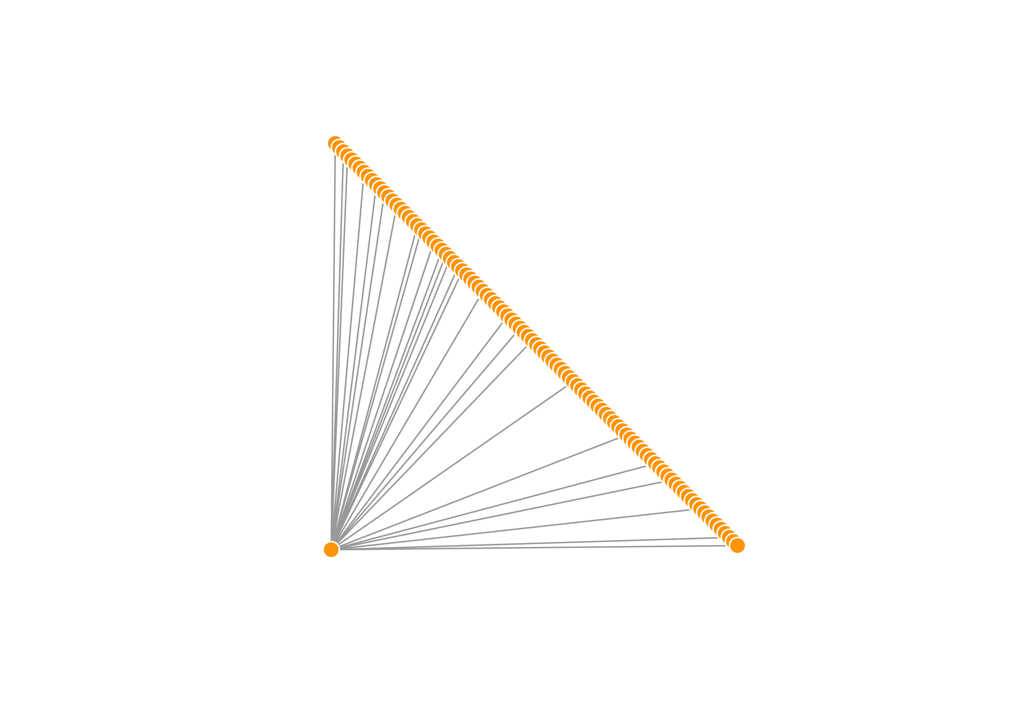

# Using tidygraph
# graph <- play_barabasi_albert(n = 100, power = 1.2)
graph %>% ggraph(., layout = l) +
  geom_edge_link(color = "grey") +
  geom_node_point(color = "orange", size = 2) +
  theme_graph()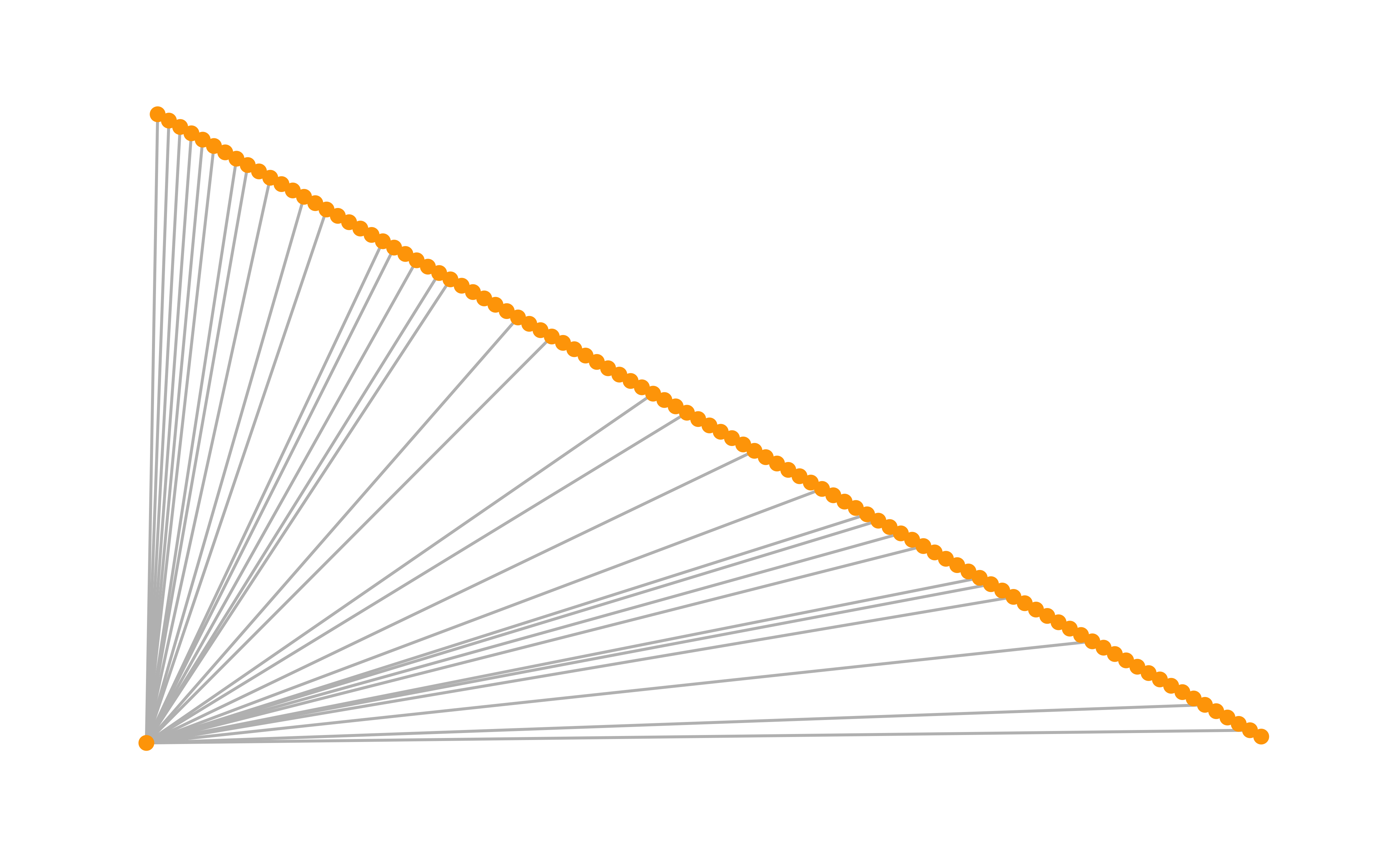

This layout is just an example and not very helpful - thankfully igraph has a number of built-in layouts, including:

Randomly placed vertices

l <- layout_randomly(net.bg)
plot(net.bg, layout = l)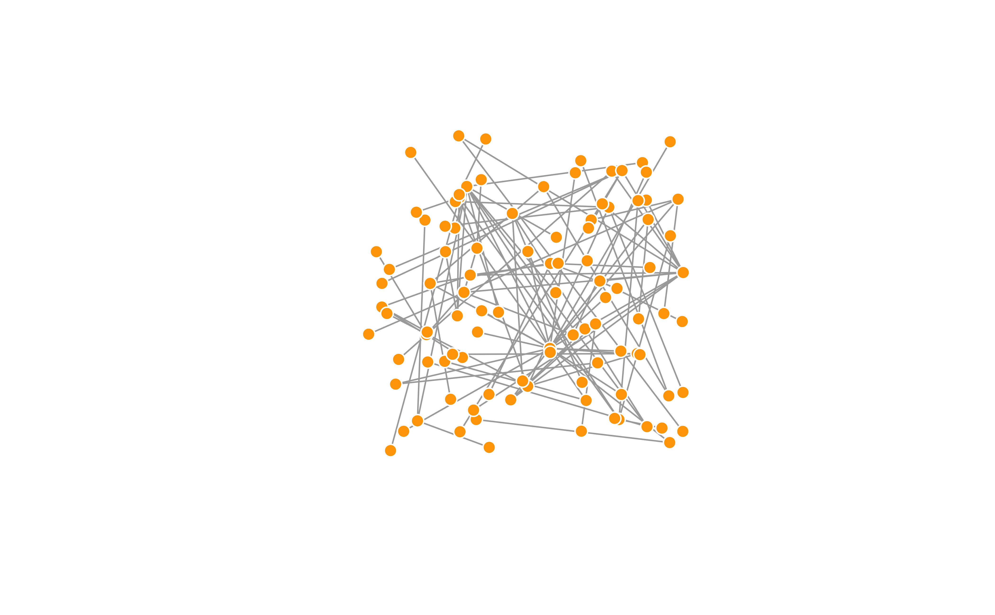

# Using tidygraph
# graph <- play_barabasi_albert(n = 100, power = 1.2)
graph %>% ggraph(., layout = layout_randomly(.)) +
  geom_edge_link0(colour = "grey") +
  geom_node_point(colour = "orange", size = 4)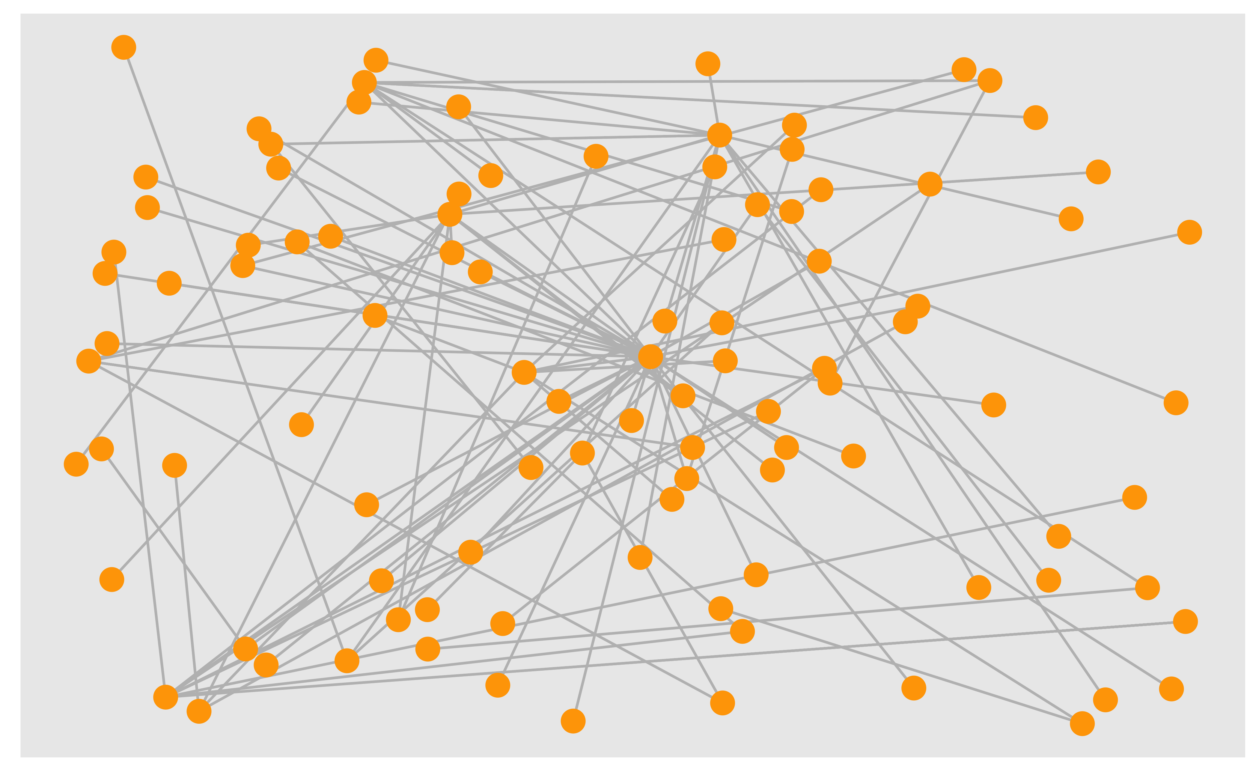

Circle layout

l <- layout_in_circle(net.bg)
plot(net.bg, layout = l)

# Using tidygraph
# graph <- play_barabasi_albert(n = 100, power = 1.2)
graph %>% ggraph(., layout = layout_in_circle(.)) +
  geom_edge_link0(colour = "grey") +
  geom_node_point(colour = "orange") +
  theme(aspect.ratio = 1)

3D sphere layout

l <- layout_on_sphere(net.bg)
plot(net.bg, layout = l)

# Using tidygraph
# graph <- play_barabasi_albert(n = 100, power = 1.2)
graph %>% ggraph(., layout = layout_on_sphere(.)) +
  geom_edge_link0(colour = "grey") +
  geom_node_point(colour = "orange")

The Fruchterman-Reingold force-directed algorithm: Nice but slow, most often used in graphs smaller than ~1000 vertices.

l <- layout_with_fr(net.bg)
plot(net.bg, layout = l)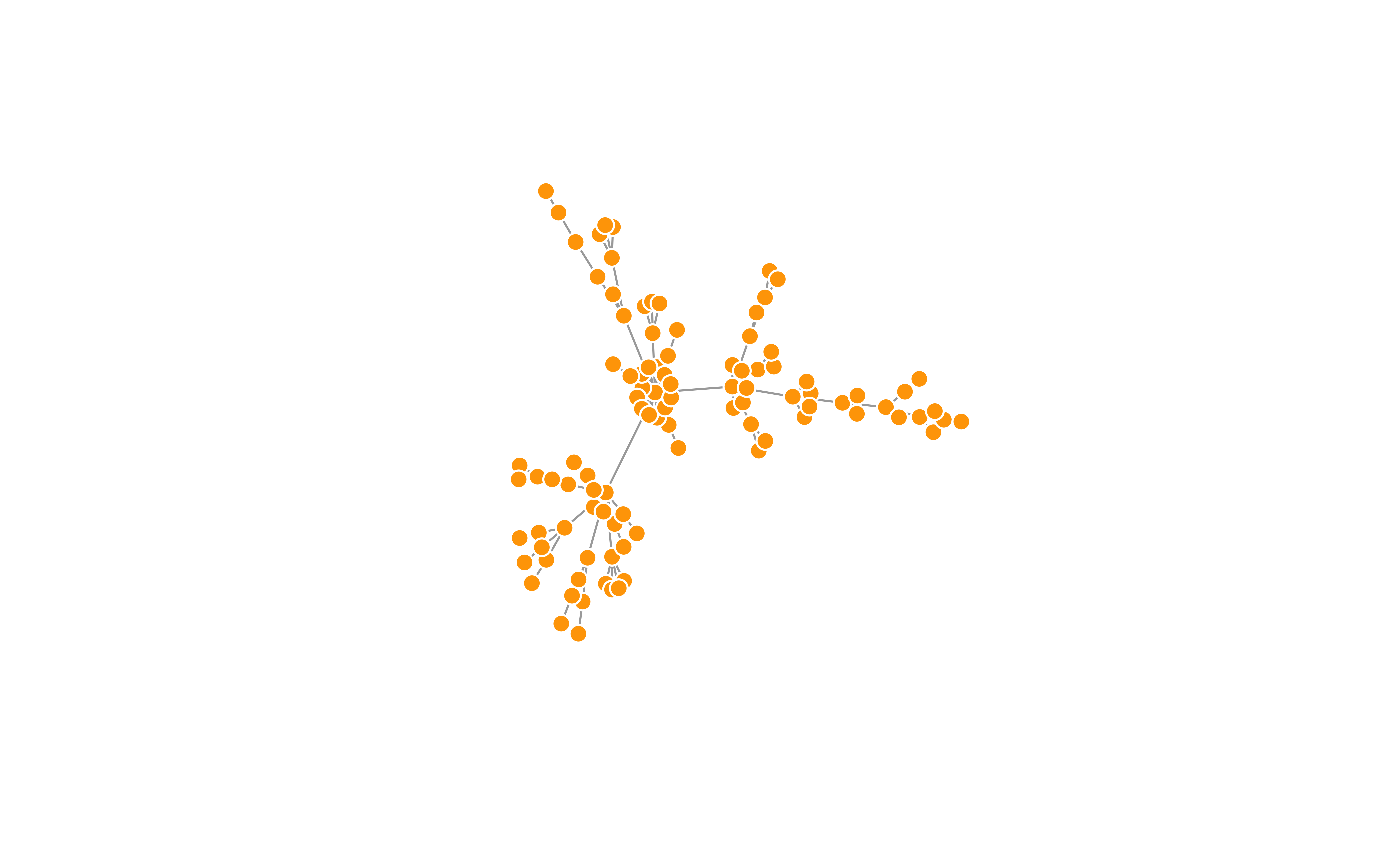

# Using tidygraph
# graph <- play_barabasi_albert(n = 100, power = 1.2)
graph %>% ggraph(., layout = layout_with_fr(.)) +
  geom_edge_link0(colour = "grey") +
  geom_node_point(colour = "orange")

You will also notice that the F-R layout is not deterministic - different runs will result in slightly different configurations. Saving the layout in l allows us to get the exact same result multiple times.

par(mfrow = c(2, 2), mar = c(1, 1, 1, 1))
plot(net.bg, layout = layout_with_fr)
plot(net.bg, layout = layout_with_fr)
plot(net.bg, layout = l)
plot(net.bg, layout = l)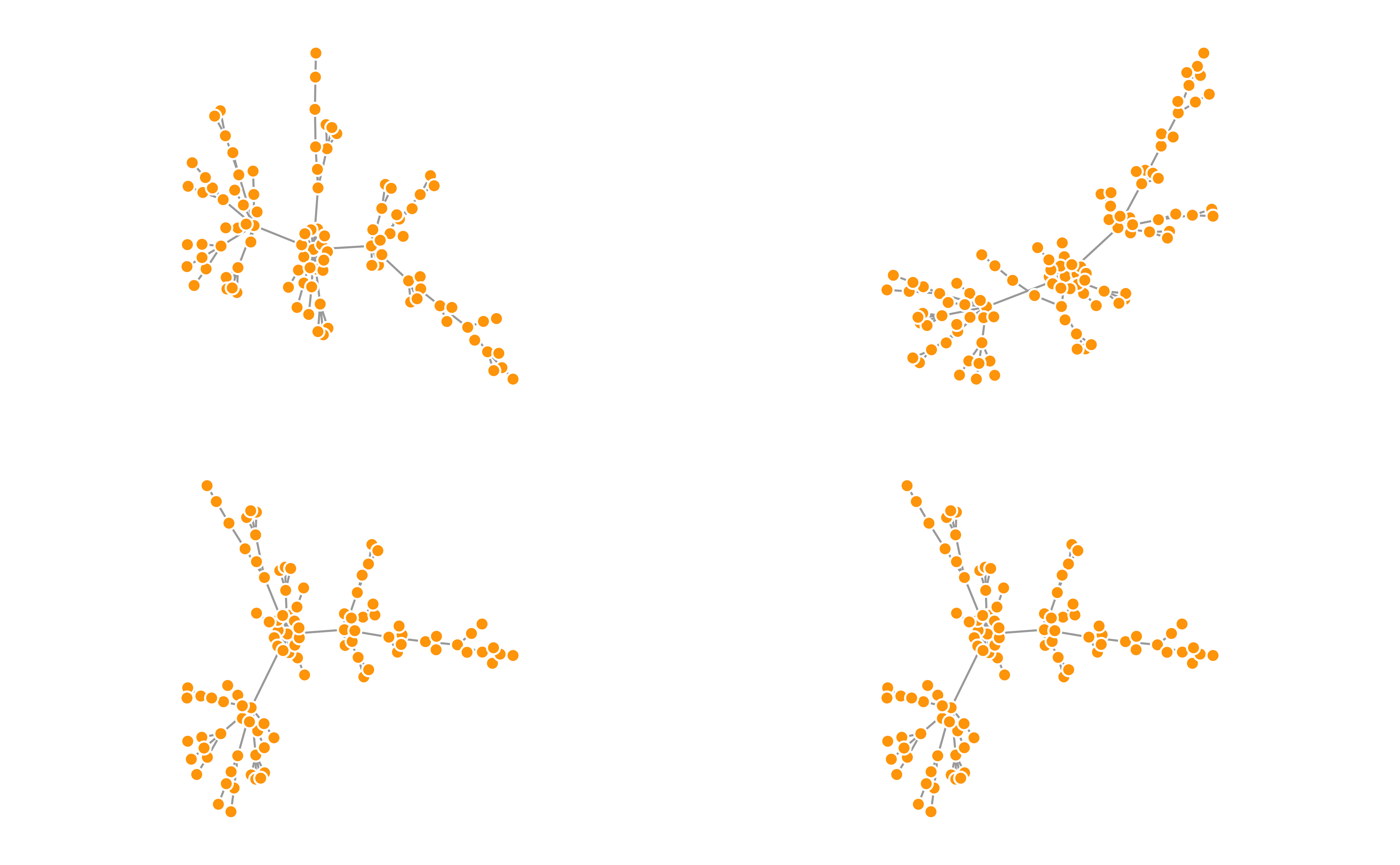

By default, the coordinates of the plots are rescaled to the [-1,1] interval for both x and y. You can change that with the parameter rescale = FALSE and rescale your plot manually by multiplying the coordinates by a scalar. You can use norm_coords to normalize the plot with the boundaries you want. This way you can create more compact or spread out layout versions.

# Get the layout coordinates:
l <- layout_with_fr(net.bg)
# Normalize them so that they are in the -1, 1 interval:
l <- norm_coords(l, ymin = -1, ymax = 1, xmin = -1, xmax = 1)

par(mfrow = c(2, 2), mar = c(0, 0, 0, 0))
plot(net.bg, rescale = F, layout = l * 0.4)
plot(net.bg, rescale = F, layout = l * 0.8)
plot(net.bg, rescale = F, layout = l * 1.2)
plot(net.bg, rescale = F, layout = l * 1.6)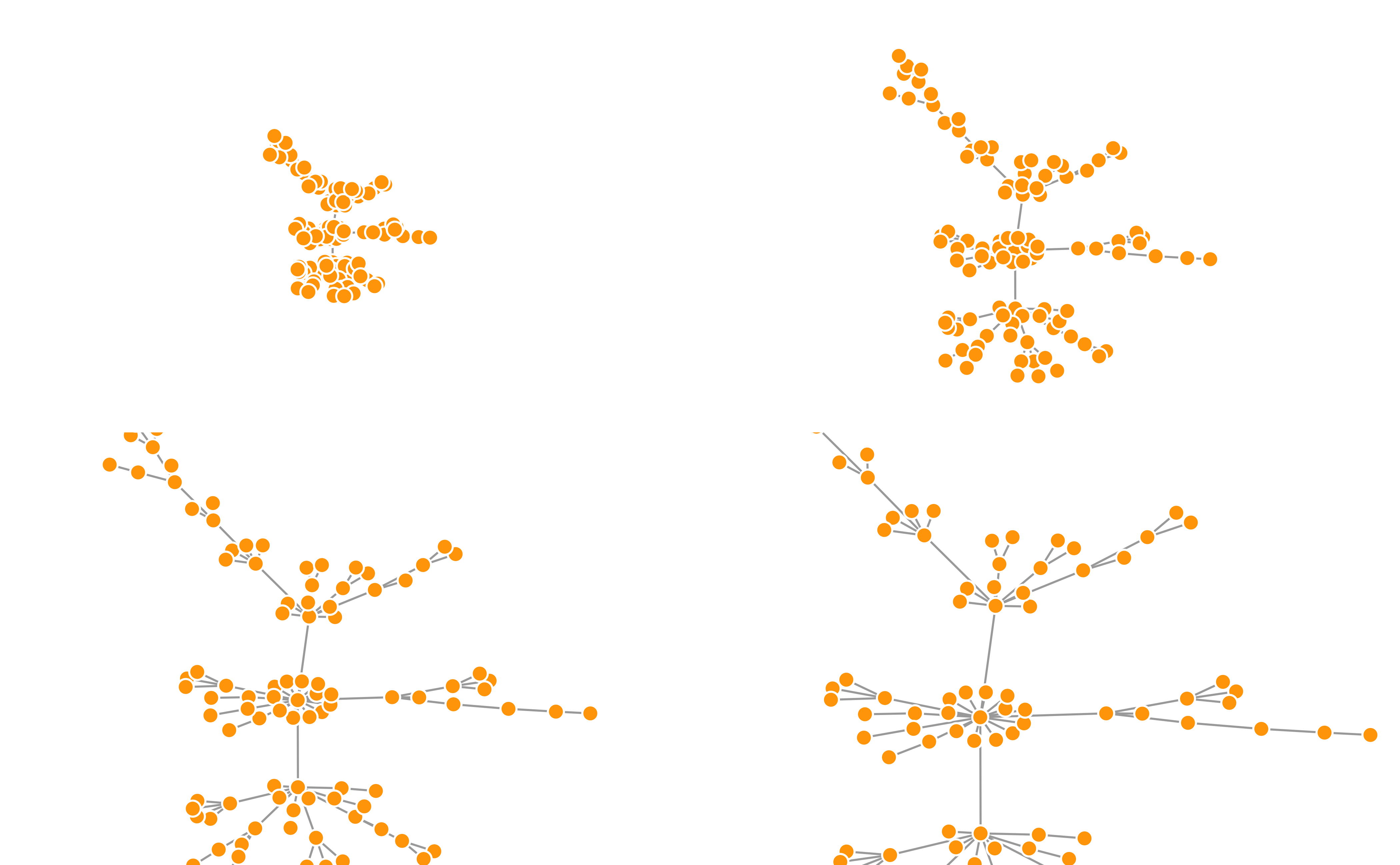

# Using tidygraph
# Can't do this with tidygraph ( multiplying layout * scalar ), it seems

Another popular force-directed algorithm that produces nice results for connected graphs is Kamada Kawai. Like Fruchterman Reingold, it attempts to minimize the energy in a spring system.

l <- layout_with_kk(net.bg)
plot(net.bg, layout = l)

# Using tidygraph
# graph <- play_barabasi_albert(n = 100, power = 1.2)
graph %>% ggraph(., layout = layout_with_kk(.)) +
  geom_edge_link0(colour = "grey") +
  geom_node_point(colour = "orange", size = 4)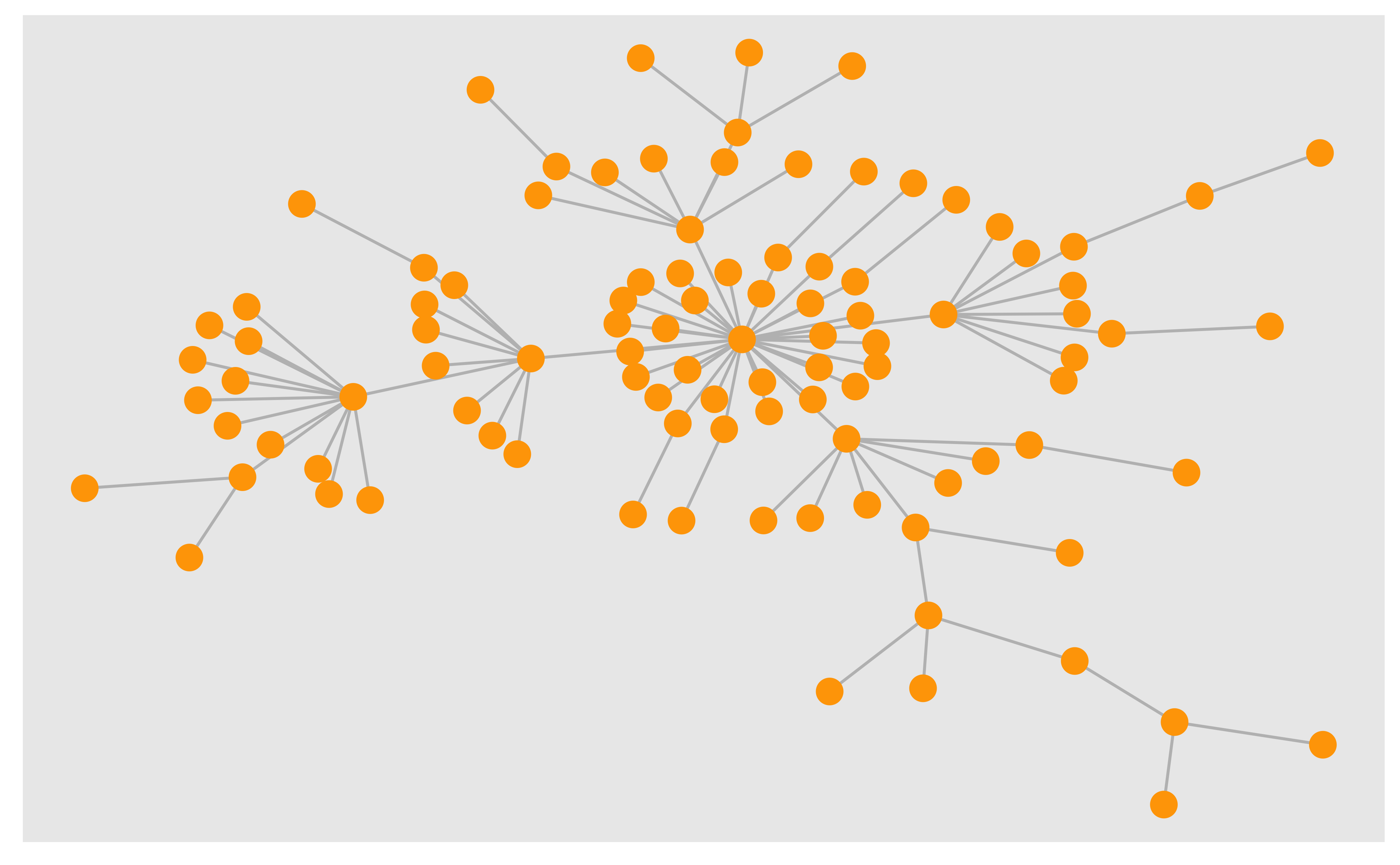

The MDS (multidimensional scaling) algorithm tries to place nodes based on some measure of similarity or distance between them. More similar/less distant nodes are placed closer to each other. By default, the measure used is based on the shortest paths between nodes in the network. That can be changed with the dist parameter.

plot(net.bg, layout = layout_with_mds)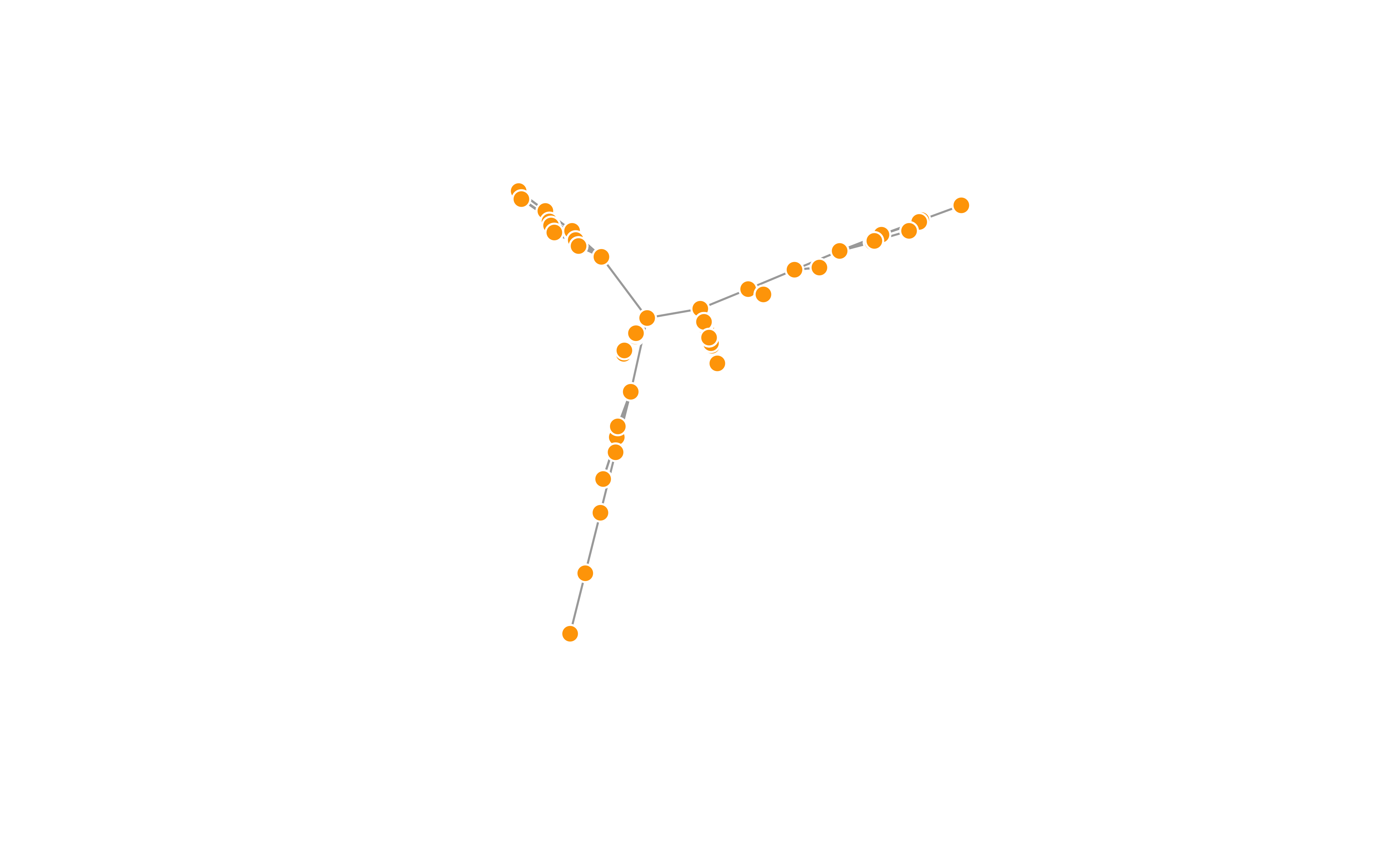

# Using tidygraph
# graph <- play_barabasi_albert(n = 100, power = 1.2)
graph %>% ggraph(., layout = layout_with_mds(.)) +
  geom_edge_link0(colour = "grey") +
  geom_node_point(colour = "orange", size = 4)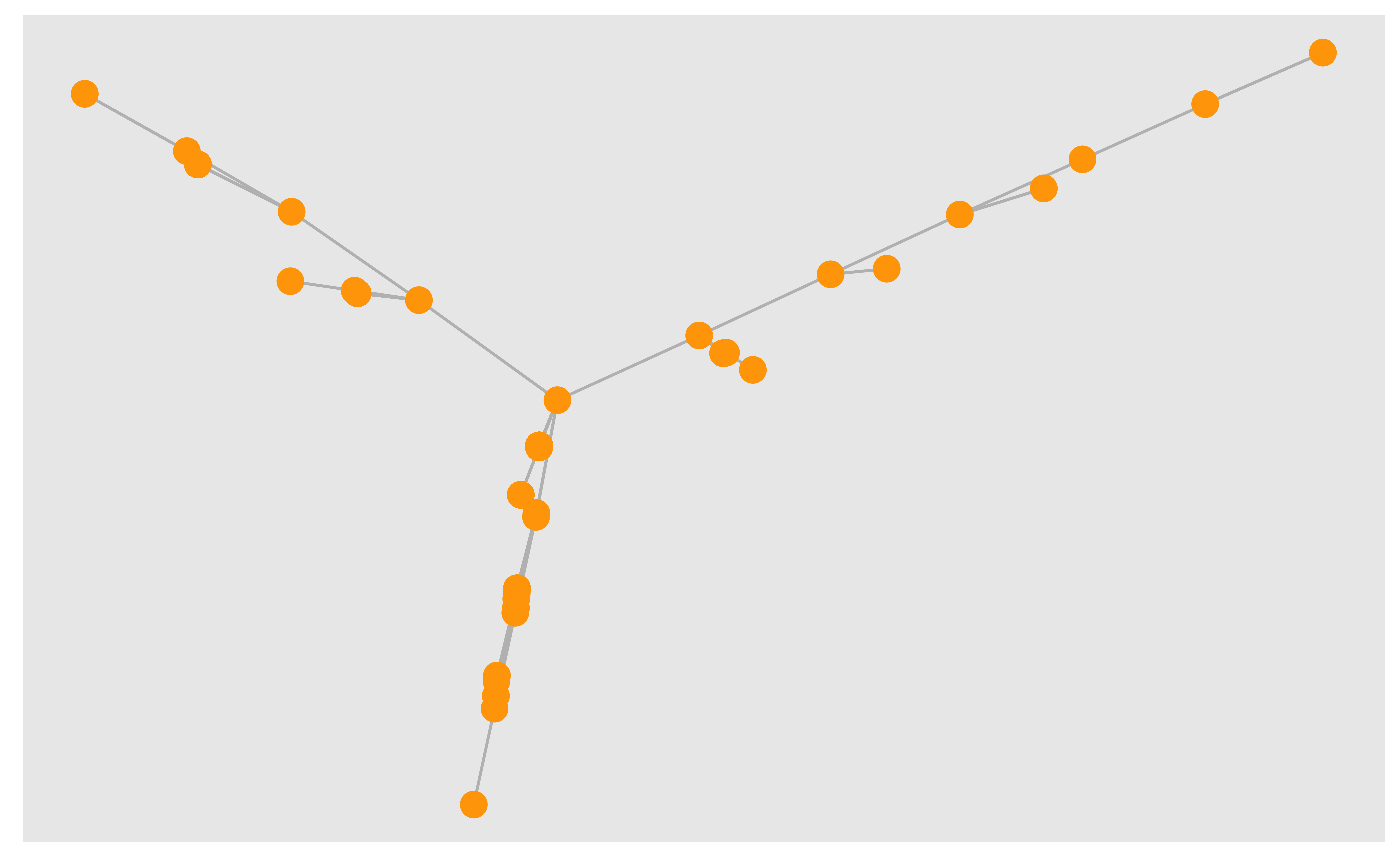

The LGL algorithm is for large connected graphs. Here you can specify a root- the node that will be placed in the middle of the layout.

plot(net.bg, layout = layout_with_lgl)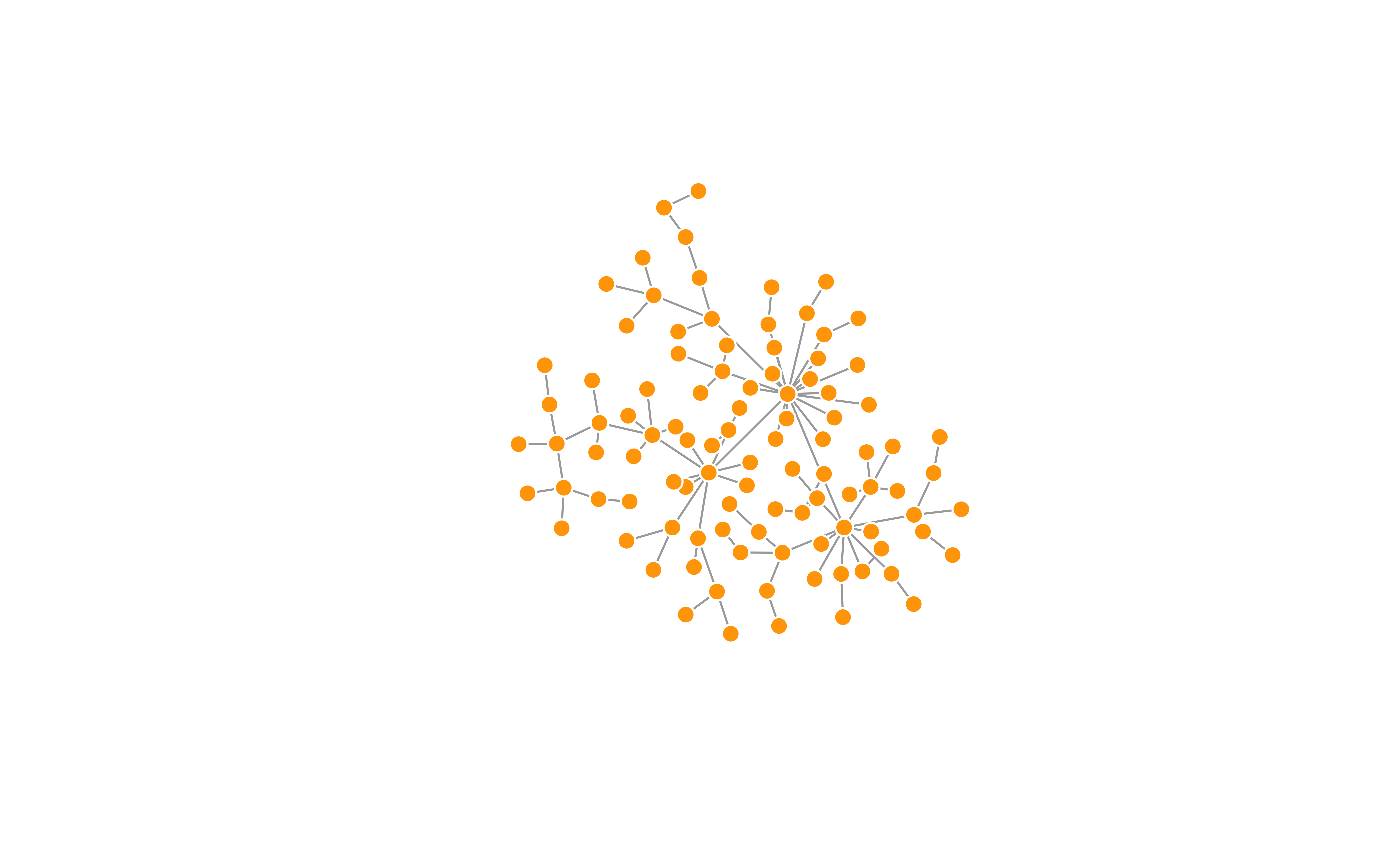

# Using tidygraph
# graph <- play_barabasi_albert(n = 100, power = 1.2)
graph %>% ggraph(., layout = layout_with_lgl(.)) +
  geom_edge_link0(colour = "grey") +
  geom_node_point(colour = "orange", size = 4)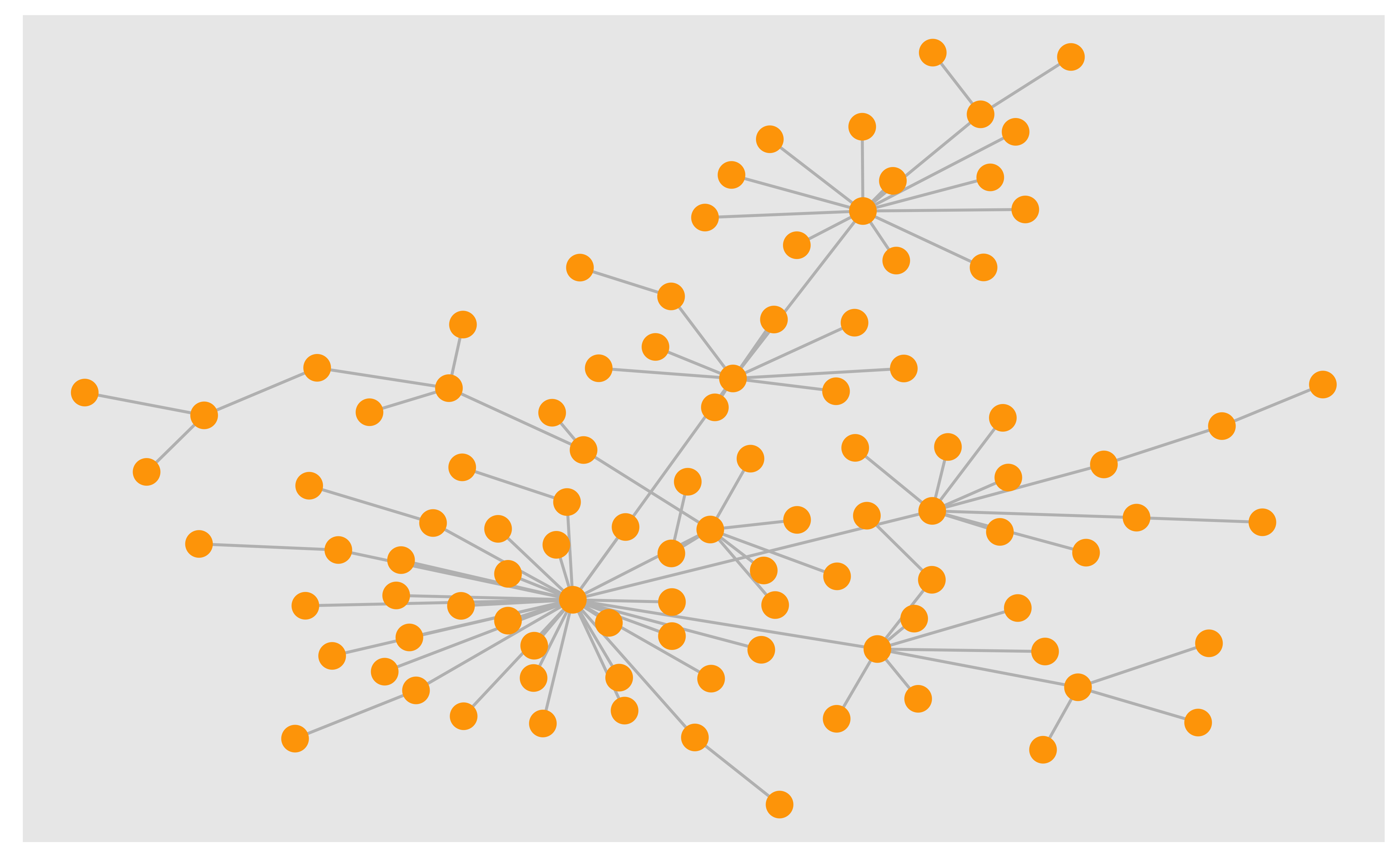

By default, igraph uses a layout called layout_nicely which selects an appropriate layout algorithm based on the properties of the graph. Check out all available layouts in igraph:

Type ?igraph::layout_ in your console

layouts <- grep("^layout_", ls("package:igraph"), value = TRUE)[-1]

# Remove layouts that do not apply to our graph.
layouts <- layouts[!grepl("bipartite|merge|norm|sugiyama|tree", layouts)]

par(mfrow = c(3, 3), mar = c(1, 1, 1, 1))

for (layout in layouts) {
  print(layout)
  l <- do.call(layout, list(net))
  plot(net, edge.arrow.mode = 0, layout = l, main = layout)
}

[1] "layout_as_star"

[1] "layout_components"

[1] "layout_in_circle"

[1] "layout_nicely"

[1] "layout_on_grid"

[1] "layout_on_sphere"

[1] "layout_randomly"

[1] "layout_with_dh"

[1] "layout_with_drl"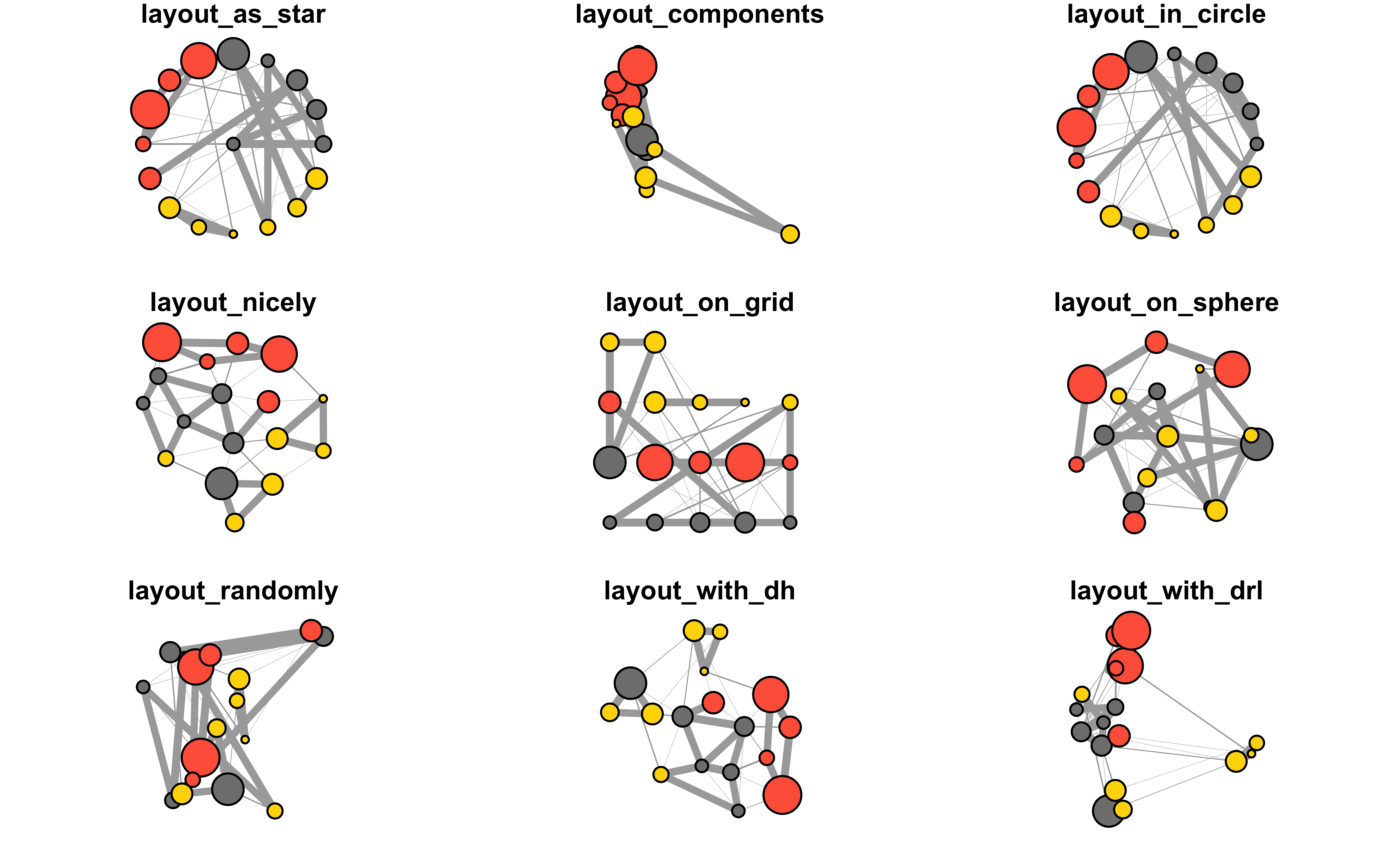

[1] "layout_with_fr"

[1] "layout_with_gem"

[1] "layout_with_graphopt"

[1] "layout_with_kk"

[1] "layout_with_lgl"

[1] "layout_with_mds"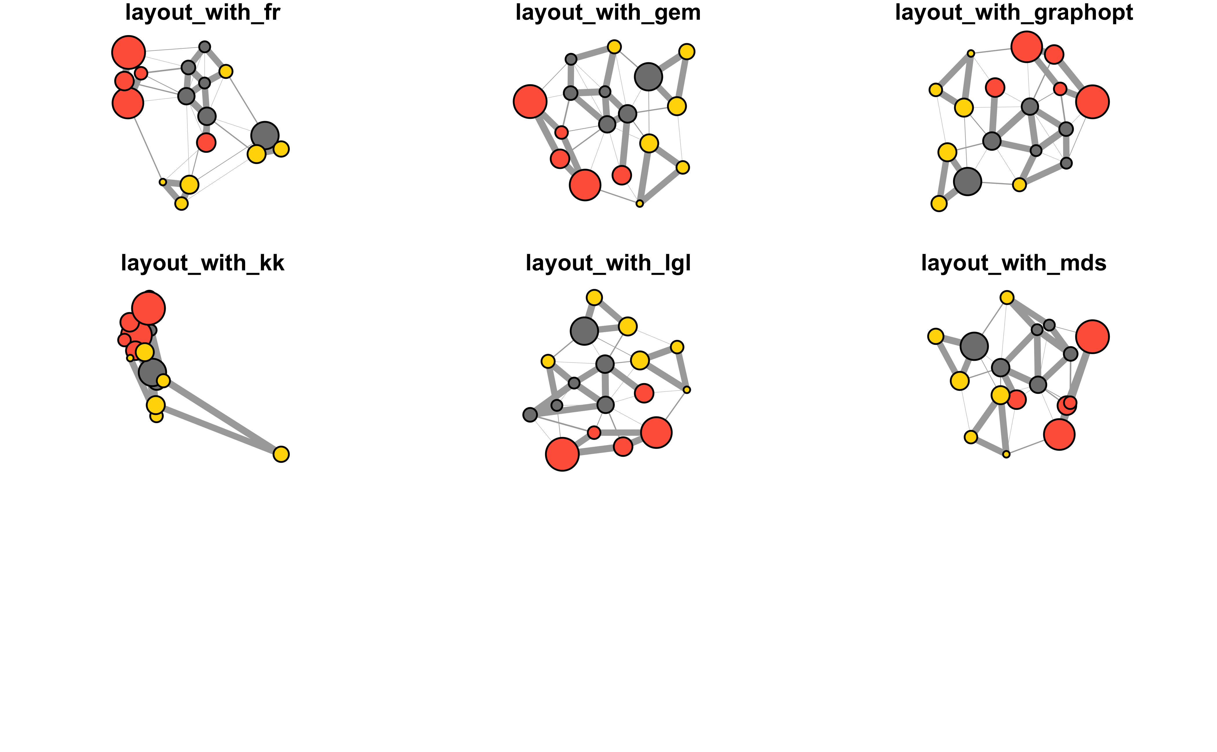

——-~~ Highlighting aspects of the network ——–

plot(net)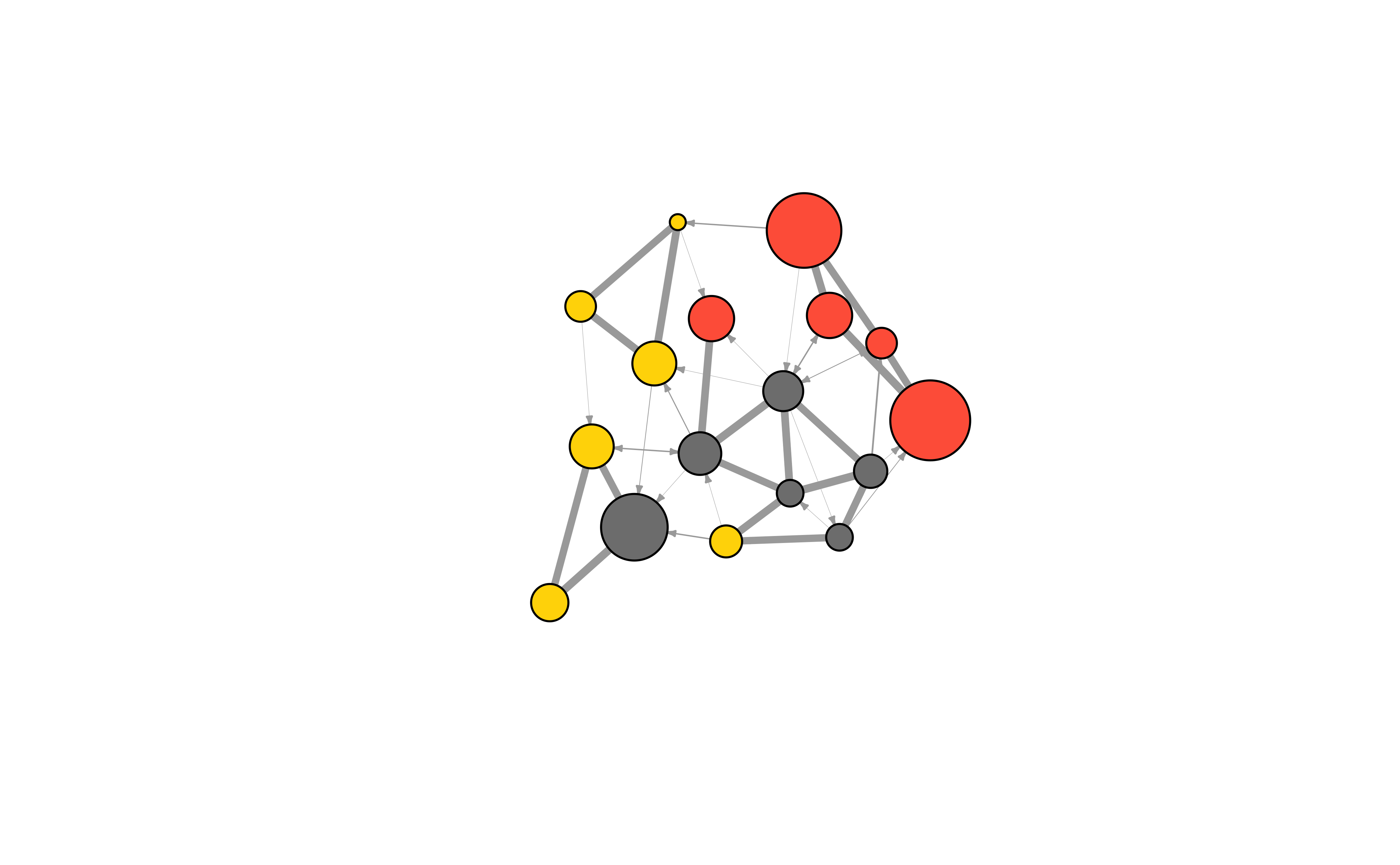

Notice that our network plot is still not too helpful. We can identify the type and size of nodes, but cannot see much about the structure since the links we’re examining are so dense. One way to approach this is to see if we can sparsify the network.

hist(links$weight)

mean(links$weight)

[1] 12.40816

sd(links$weight)

[1] 9.905635

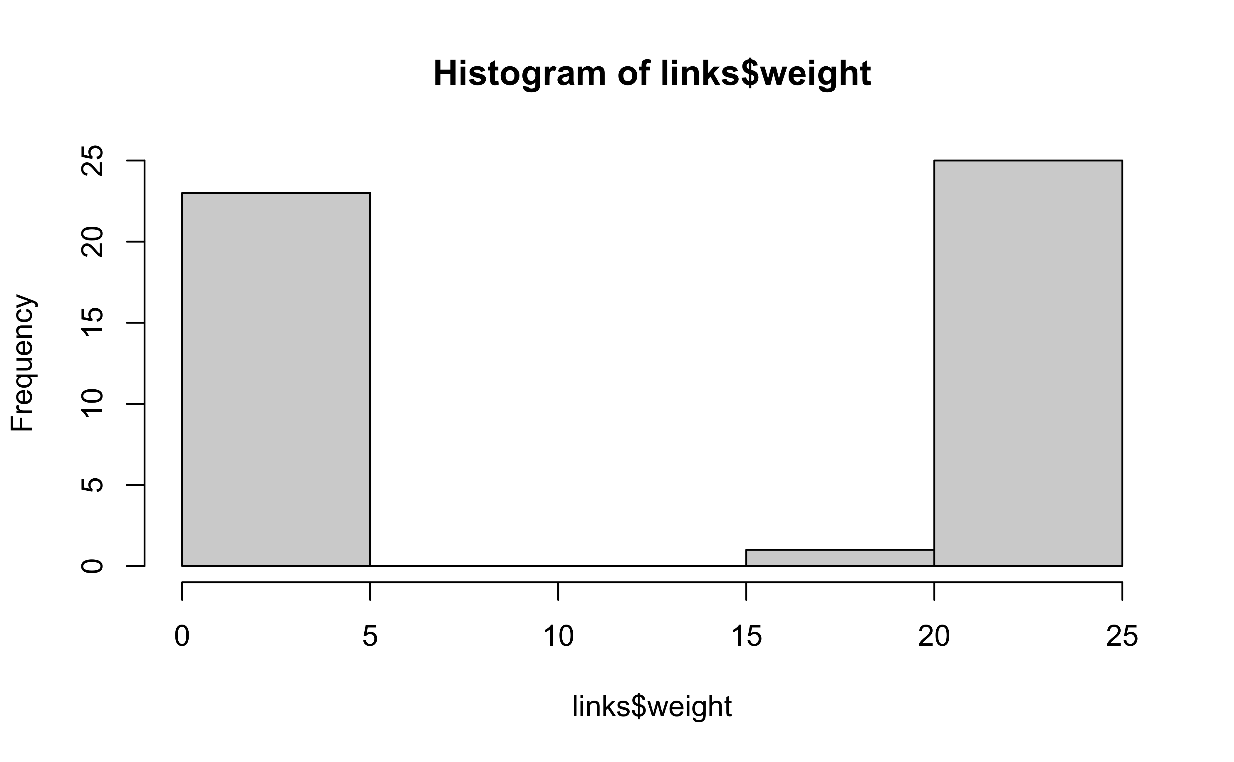
There are more sophisticated ways to extract the key edges, but for the purposes of this exercise we’ll only keep ones that have weight higher than the mean for the network. We can delete edges using delete_edges(net, edges) (or, by the way, add edges with add_edges(net, edges) )

cut.off <- mean(links$weight)
net.sp <- delete_edges(net, E(net)[weight < cut.off])
plot(net.sp, layout = layout_with_kk)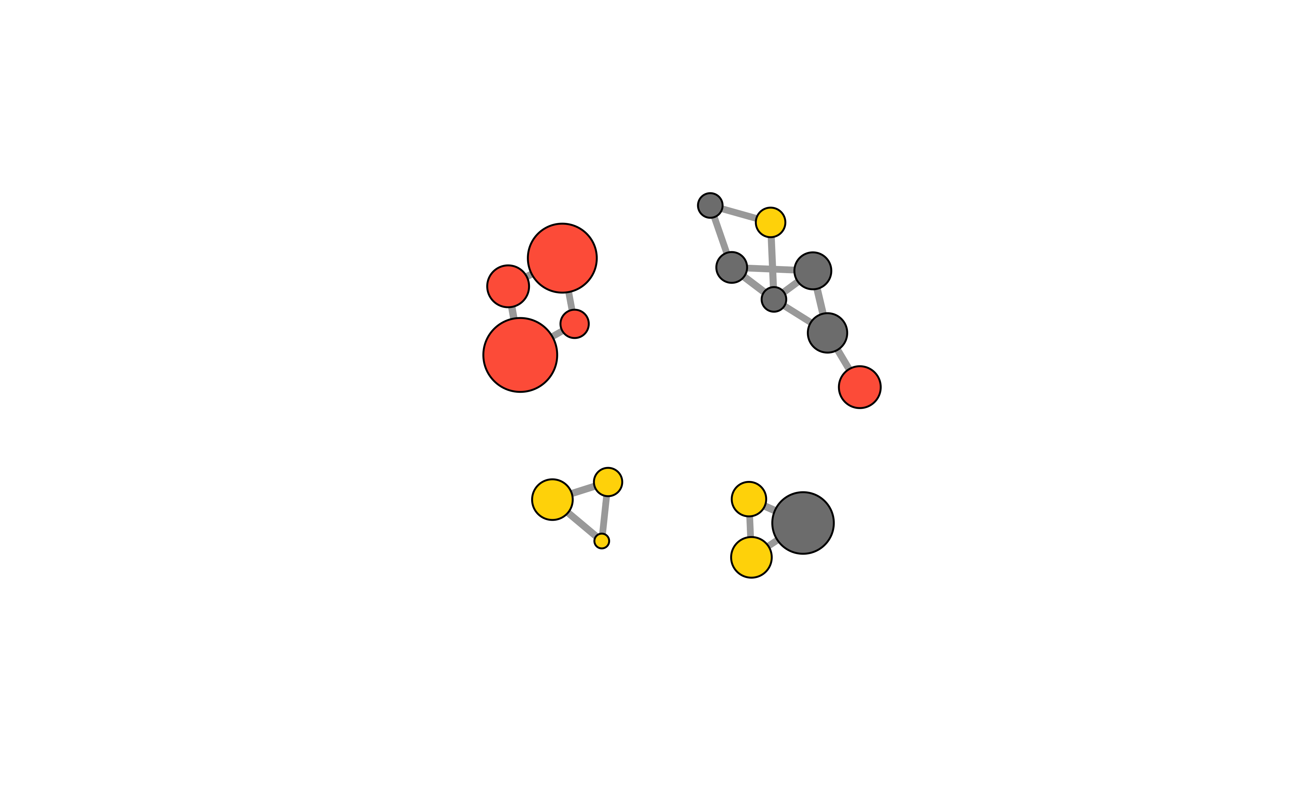

# Using tidygraph
graph <- tbl_graph(nodes, links, directed = TRUE)
graph

# A tbl_graph: 17 nodes and 49 edges
#
# A directed multigraph with 1 component
#
# Node Data: 17 × 5 (active)
   id    media               media.type type.label audience.size
   <chr> <chr>                    <int> <chr>              <int>
 1 s01   NY Times                     1 Newspaper             20
 2 s02   Washington Post              1 Newspaper             25
 3 s03   Wall Street Journal          1 Newspaper             30
 4 s04   USA Today                    1 Newspaper             32
 5 s05   LA Times                     1 Newspaper             20
 6 s06   New York Post                1 Newspaper             50
 7 s07   CNN                          2 TV                    56
 8 s08   MSNBC                        2 TV                    34
 9 s09   FOX News                     2 TV                    60
10 s10   ABC                          2 TV                    23
11 s11   BBC                          2 TV                    34
12 s12   Yahoo News                   3 Online                33
13 s13   Google News                  3 Online                23
14 s14   Reuters.com                  3 Online                12
15 s15   NYTimes.com                  3 Online                24
16 s16   WashingtonPost.com           3 Online                28
17 s17   AOL.com                      3 Online                33
#
# Edge Data: 49 × 4
   from    to type      weight
  <int> <int> <chr>      <int>
1     1     2 hyperlink     22
2     1     3 hyperlink     22
3     1     4 hyperlink     21
# ℹ 46 more rows

graph %>%
  activate(nodes) %>%
  mutate(size = centrality_degree()) %>%
  # New stuff here
  activate(edges) %>%
  filter(weight >= mean(weight)) %>%
  ggraph(., layout = "kk") +
  geom_edge_link(
    aes(width = weight),
    color = "grey80",
    end_cap = circle(.2, "cm"),
    arrow = arrow(
      type = "closed",
      ends = "last",
      length = unit(1, "mm")
    )
  ) +
  geom_node_point(
    aes(
      fill = type.label,
      size = size
    ),
    shape = 21,
    color = "black"
  ) +
  scale_fill_manual(
    name = "Media Type",
    values = c("grey50", "gold", "tomato"),
    guide = "legend"
  ) +

  scale_edge_width(range = c(0.2, 1.5), guide = "none") +
  scale_size_continuous("Degree", range = c(2, 16)) +
  # not "limits"!
  guides(fill = guide_legend(override.aes = list(
    pch = 21,
    size = 4
  )))

Another way to think about this is to plot the two tie types (hyperlinks and mentions) separately. We will do that in section 5 of this tutorial: Plotting multiplex networks.

Community Detection

We can also try to make the network map more useful by showing the communities within it.

# Community detection (by optimizing modularity over partitions):
clp <- cluster_optimal(net)
class(clp)

[1] "communities"

clp

IGRAPH clustering optimal, groups: 4, mod: 0.6
+ groups:
  $`1`
  [1] "s01" "s02" "s03" "s04" "s05" "s11" "s15"
  
  $`2`
  [1] "s06" "s16" "s17"
  
  $`3`
  [1] "s07" "s08" "s09" "s10"
  
  $`4`
  + ... omitted several groups/vertices

clp$membership

 [1] 1 1 1 1 1 2 3 3 3 3 1 4 4 4 1 2 2

Community detection returns an object of class “communities” which igraph knows how to plot:

plot(clp, net)

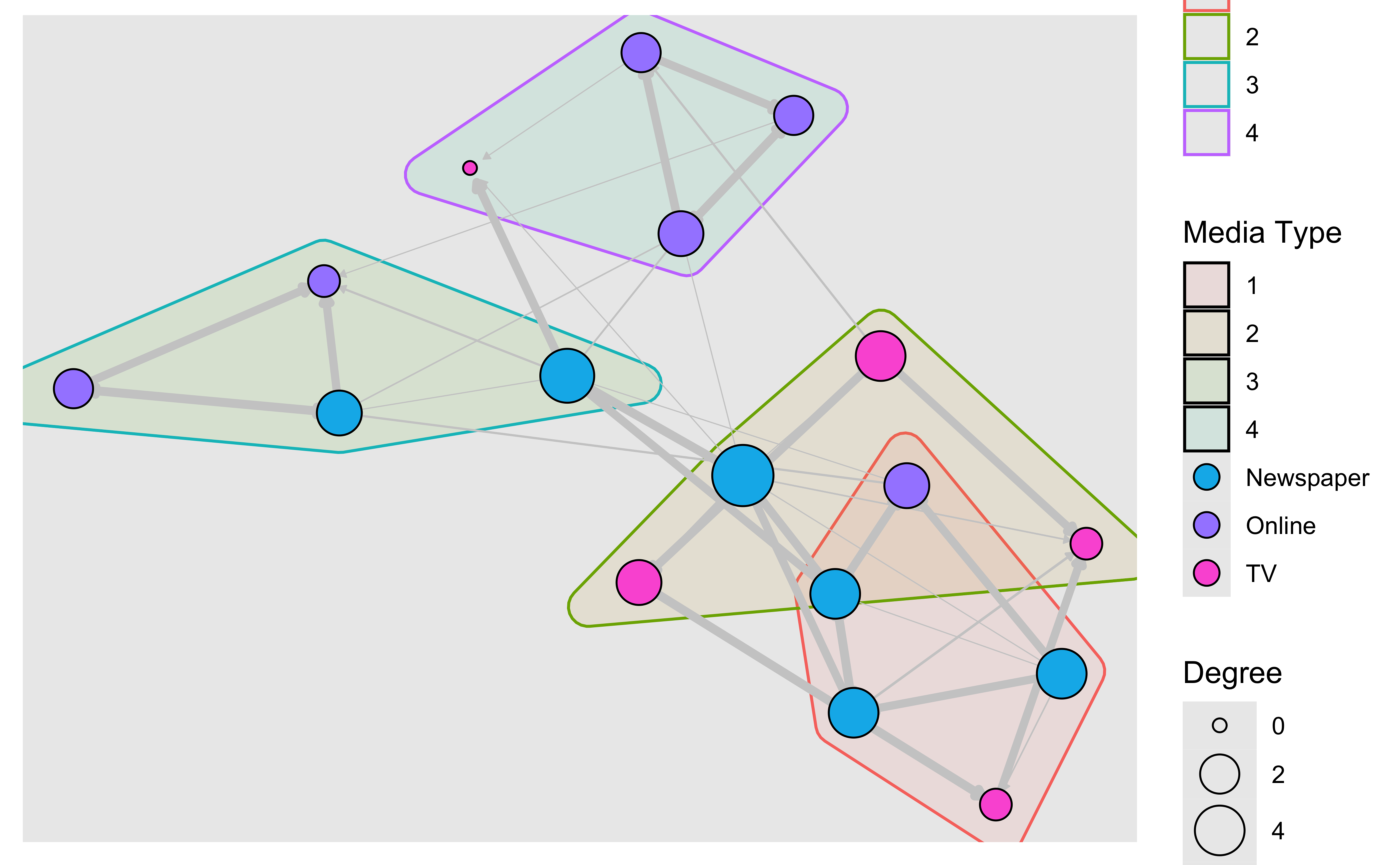
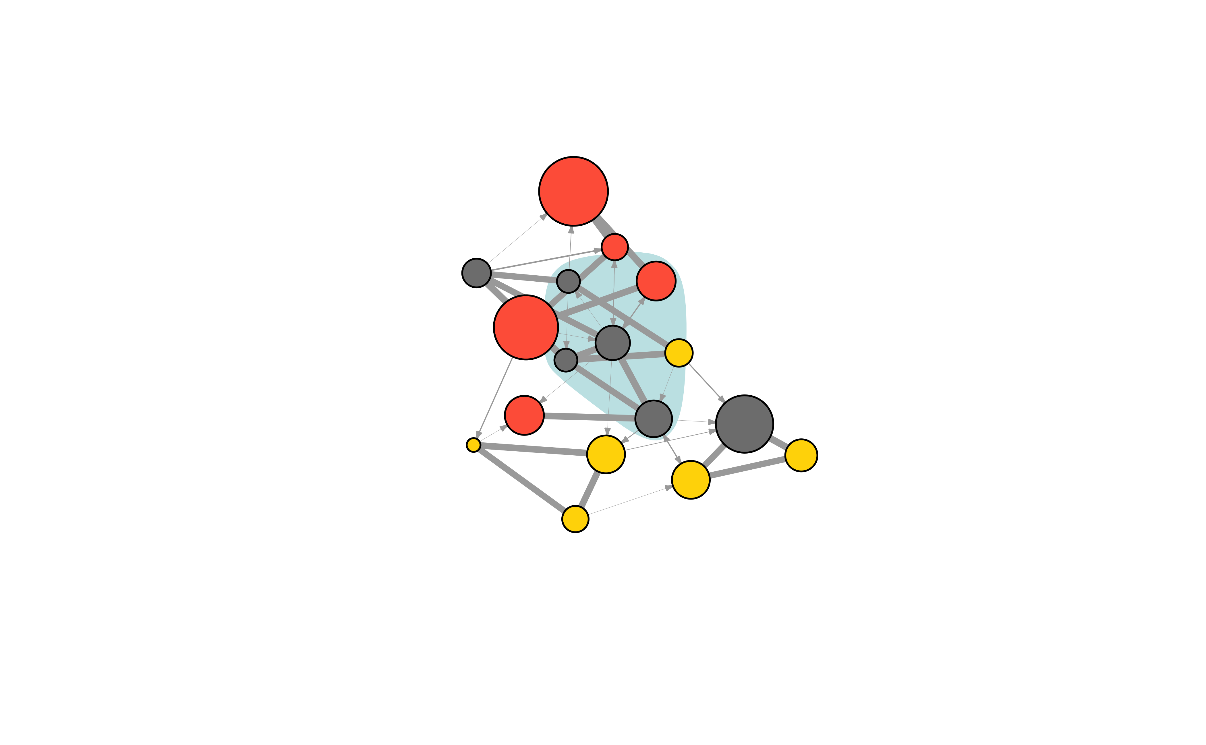
To plot communities using the tidygraph approach, I have taken help from the ggforce package. This package allows drawing of hull shapes around specific sets of points. Here goes:

# Using tidygraph
# And ggforce
library(ggforce)
graph <- tbl_graph(nodes, links, directed = TRUE)
graph <- graph %>%
  activate(nodes) %>%
  mutate(size = centrality_degree()) %>%
  # new stuff
  mutate(community = as.factor(tidygraph::group_optimal()))

# Need to pre-compute layout coordinates to pass to ggforce
# To create a hull around each community
layout_go <- layout_with_graphopt(graph)

ggraph(graph, layout = layout_go) +

  # new stuff
  # need to pass x and y coordinates of nodes to `geom_mark_hull`
  # Hull colour is `community`
  #
  ggforce::geom_mark_hull(aes(
    x = layout_go[, 1],
    y = layout_go[, 2],
    color = community, fill = community
  ), alpha = 0.1) +

  geom_edge_link(
    aes(width = weight),
    color = "grey80",
    end_cap = circle(.2, "cm"),
    arrow = arrow(
      type = "closed",
      ends = "last",
      length = unit(1, "mm")
    )
  ) +
  geom_node_point(
    aes(
      fill = type.label,
      size = size
    ),
    shape = 21,
    color = "black"
  ) +
  scale_edge_width(range = c(0.2, 1.5), guide = "none") +
  scale_size_continuous("Degree", range = c(2, 10)) +
  scale_fill_discrete("Media Type") +
  scale_colour_discrete("Community") +
  guides(fill = guide_legend(override.aes = list(
    pch = 21,
    size = 4
  )))

We can also plot the communities without relying on their built-in plot:

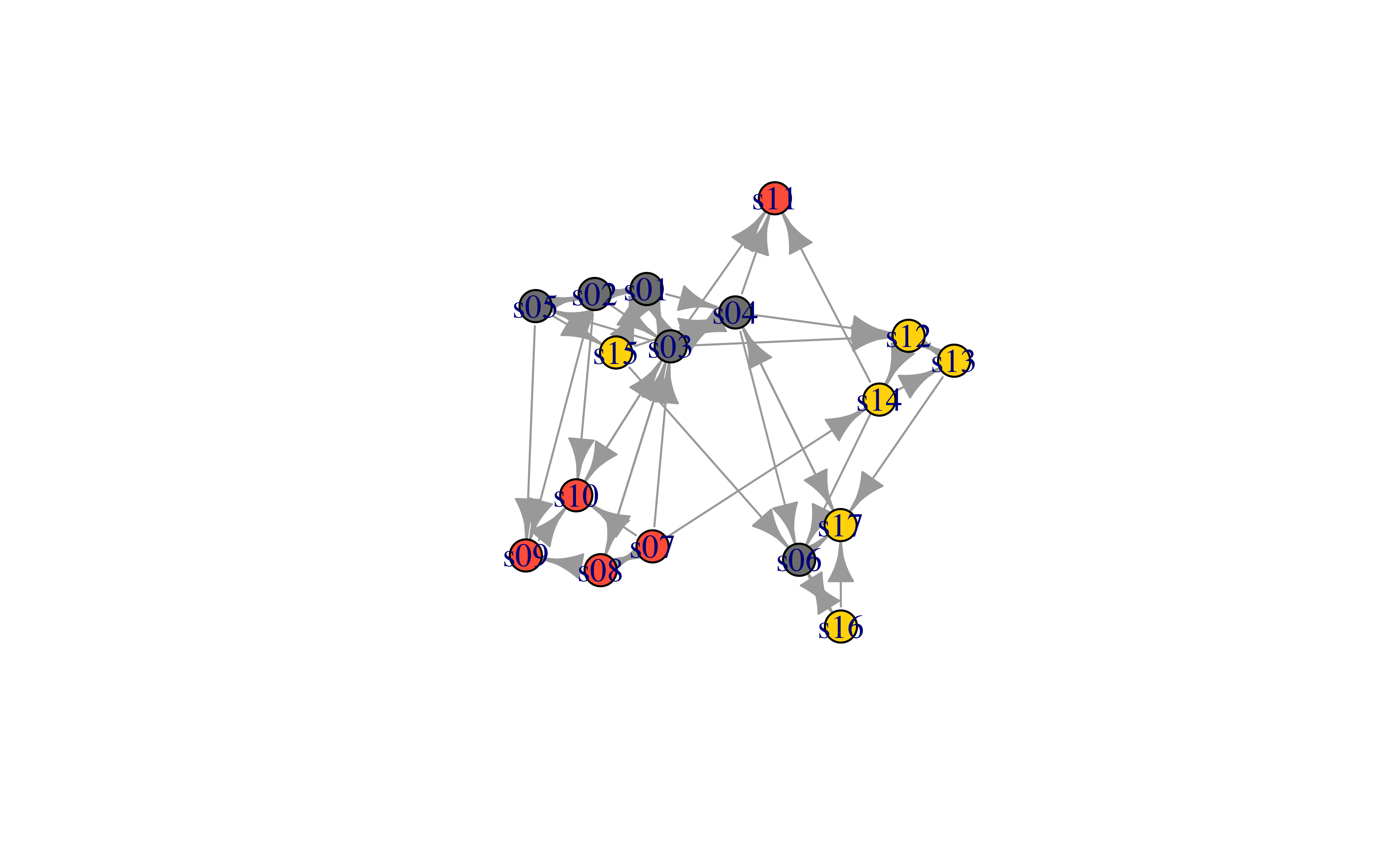
V(net)$community <- clp$membership
colrs <-
  adjustcolor(c("gray50", "tomato", "gold", "yellowgreen"), alpha = .6)
plot(net, vertex.color = colrs[V(net)$community])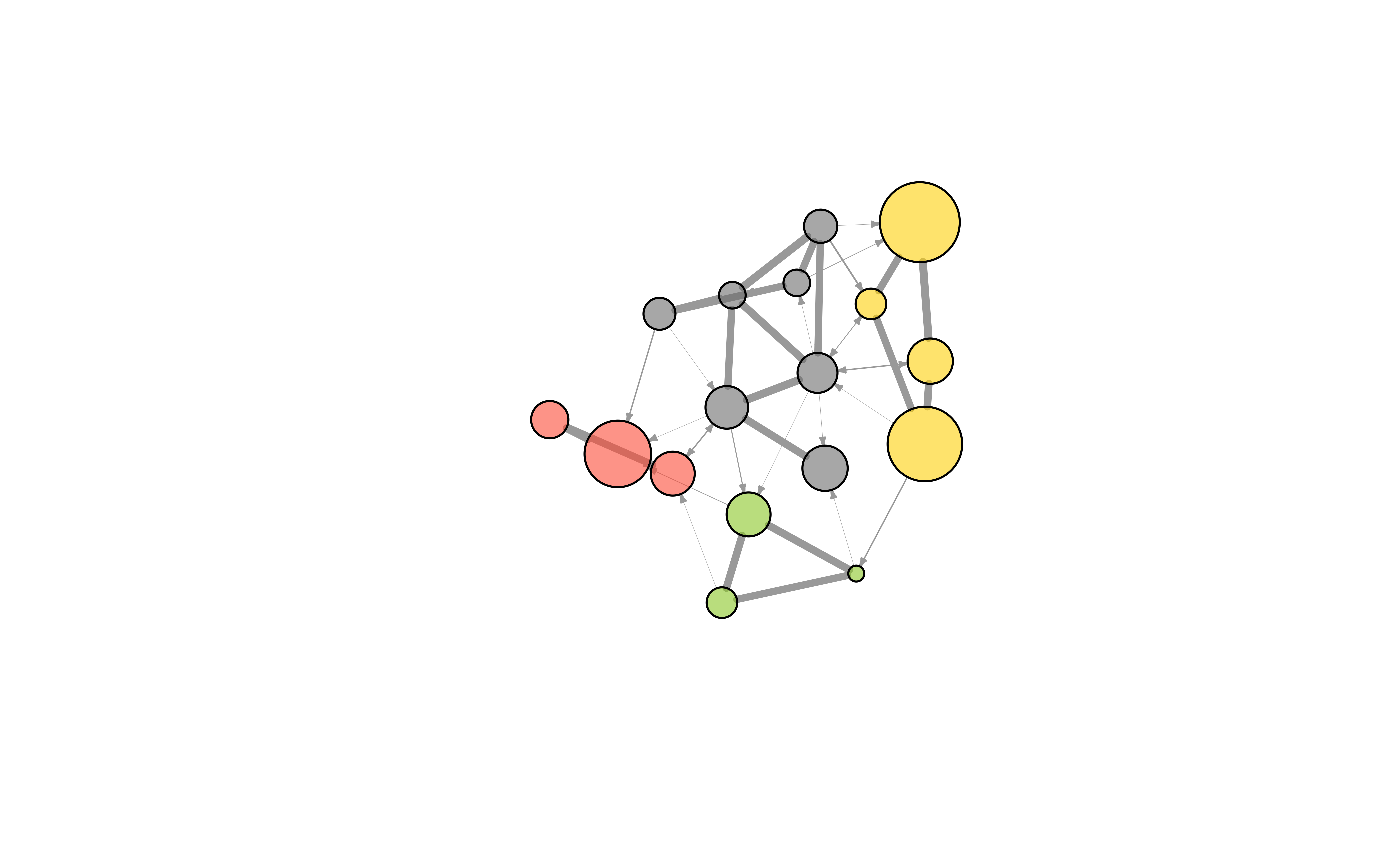

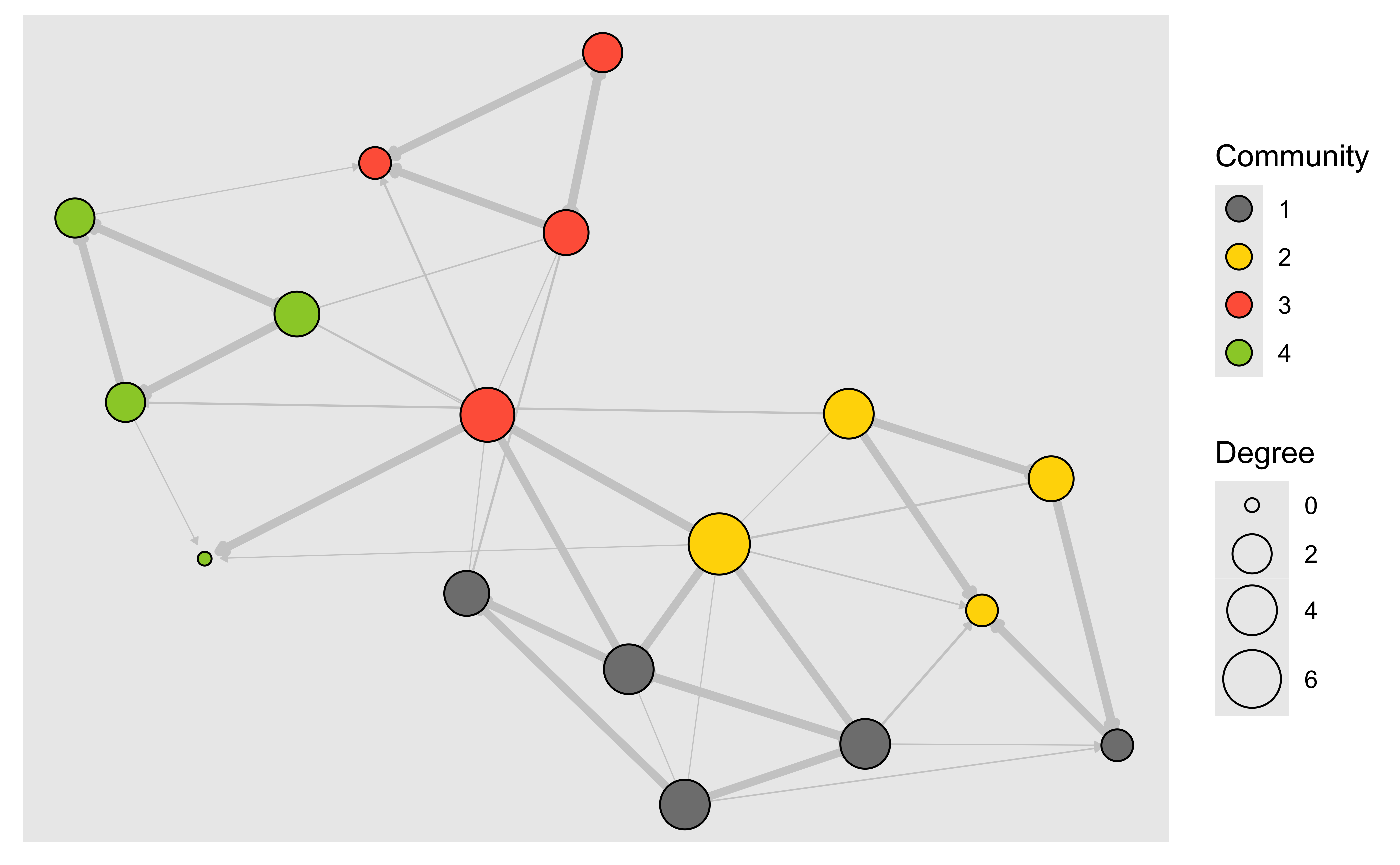
# using tidygraph
# All clustering algorithms from igraph is available in tidygraph using the group_* prefix. All of these functions return an integer vector with nodes (or edges) sharing the same integer being grouped together.
graph <- tbl_graph(nodes, links, directed = TRUE)
graph

# A tbl_graph: 17 nodes and 49 edges
#
# A directed multigraph with 1 component
#
# Node Data: 17 × 5 (active)
   id    media               media.type type.label audience.size
   <chr> <chr>                    <int> <chr>              <int>
 1 s01   NY Times                     1 Newspaper             20
 2 s02   Washington Post              1 Newspaper             25
 3 s03   Wall Street Journal          1 Newspaper             30
 4 s04   USA Today                    1 Newspaper             32
 5 s05   LA Times                     1 Newspaper             20
 6 s06   New York Post                1 Newspaper             50
 7 s07   CNN                          2 TV                    56
 8 s08   MSNBC                        2 TV                    34
 9 s09   FOX News                     2 TV                    60
10 s10   ABC                          2 TV                    23
11 s11   BBC                          2 TV                    34
12 s12   Yahoo News                   3 Online                33
13 s13   Google News                  3 Online                23
14 s14   Reuters.com                  3 Online                12
15 s15   NYTimes.com                  3 Online                24
16 s16   WashingtonPost.com           3 Online                28
17 s17   AOL.com                      3 Online                33
#
# Edge Data: 49 × 4
   from    to type      weight
  <int> <int> <chr>      <int>
1     1     2 hyperlink     22
2     1     3 hyperlink     22
3     1     4 hyperlink     21
# ℹ 46 more rows

graph %>%
  activate(nodes) %>%
  mutate(size = centrality_degree()) %>%
  # new stuff
  mutate(community = as.factor(tidygraph::group_optimal())) %>%
  ggraph(., layout = "graphopt") +
  geom_edge_link(
    aes(width = weight),
    color = "grey80",
    end_cap = circle(.2, "cm"),
    # clears an area near the node

    arrow = arrow(
      type = "closed",
      ends = "last",
      length = unit(1, "mm")
    )
  ) +
  geom_node_point(
    aes(
      fill = community,
      size = size
    ),
    shape = 21,
    color = "black"
  ) +
  scale_fill_manual(
    name = "Community",
    values = c("grey50", "gold", "tomato", "yellowgreen"),
    guide = "legend"
  ) +

  scale_edge_width(range = c(0.2, 1.5), guide = "none") +
  scale_size_continuous("Degree", range = c(2, 10)) +
  guides(fill = guide_legend(override.aes = list(
    pch = 21,
    size = 4
  )))

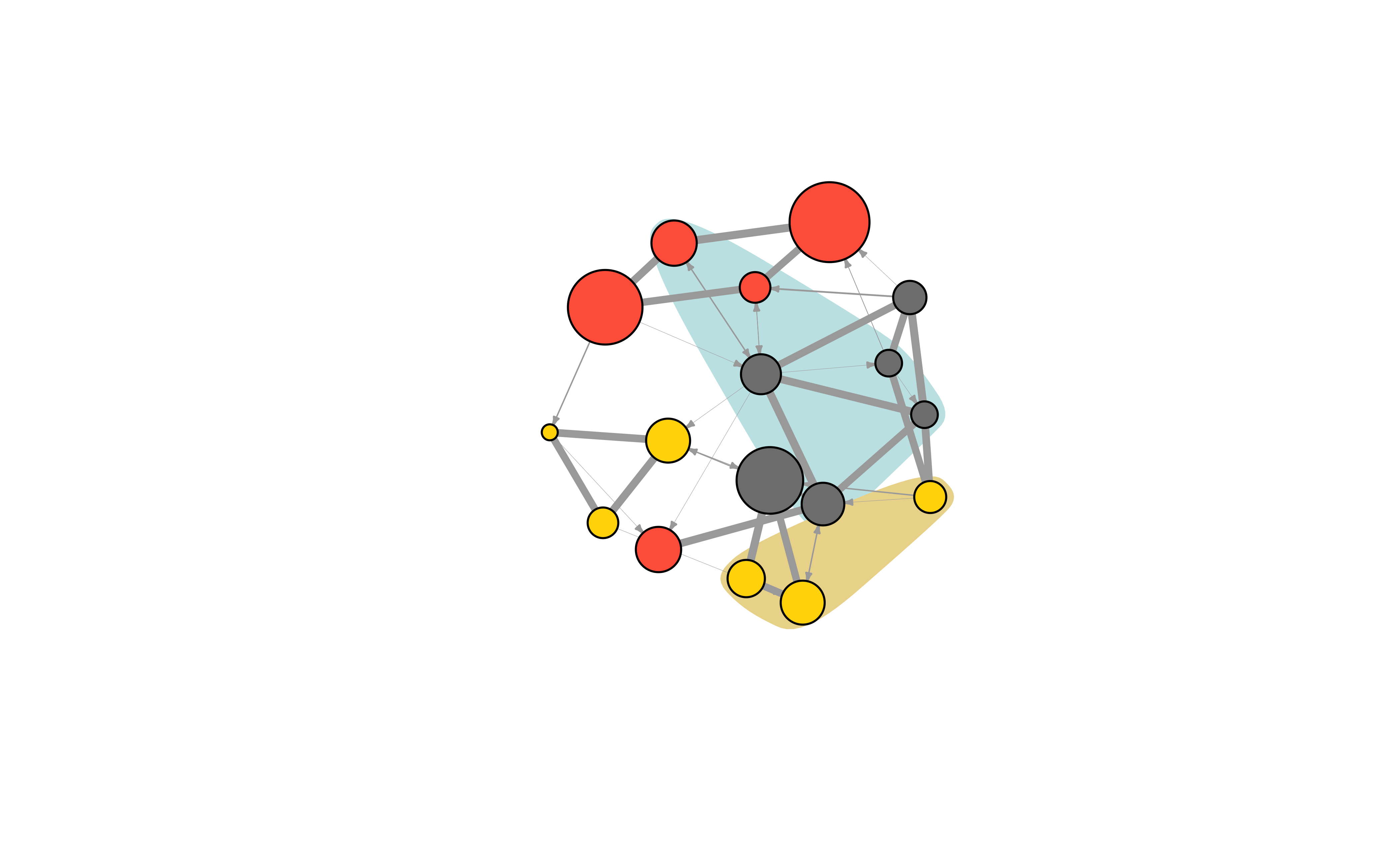
——-~~ Highlighting specific nodes or links ——–

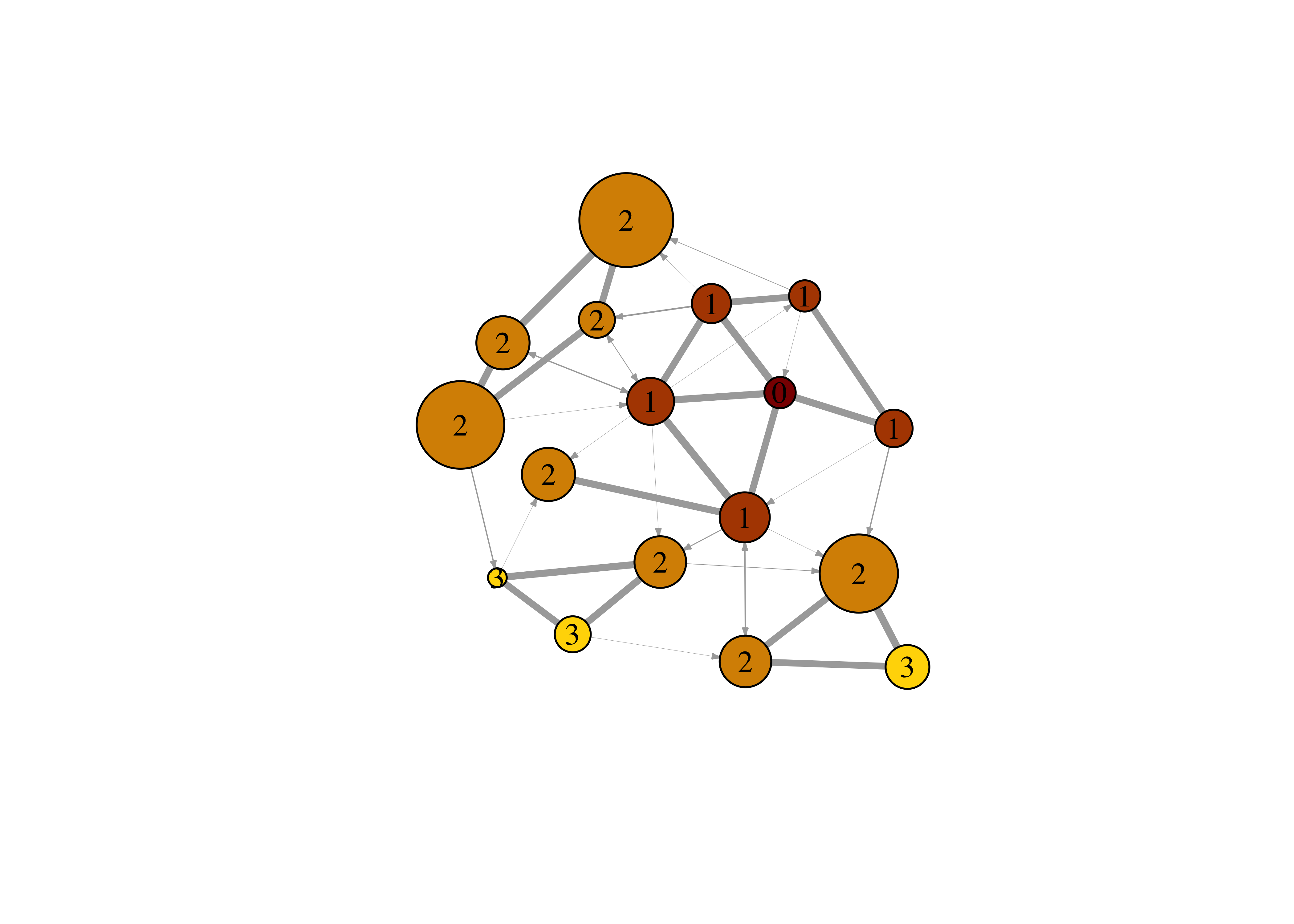
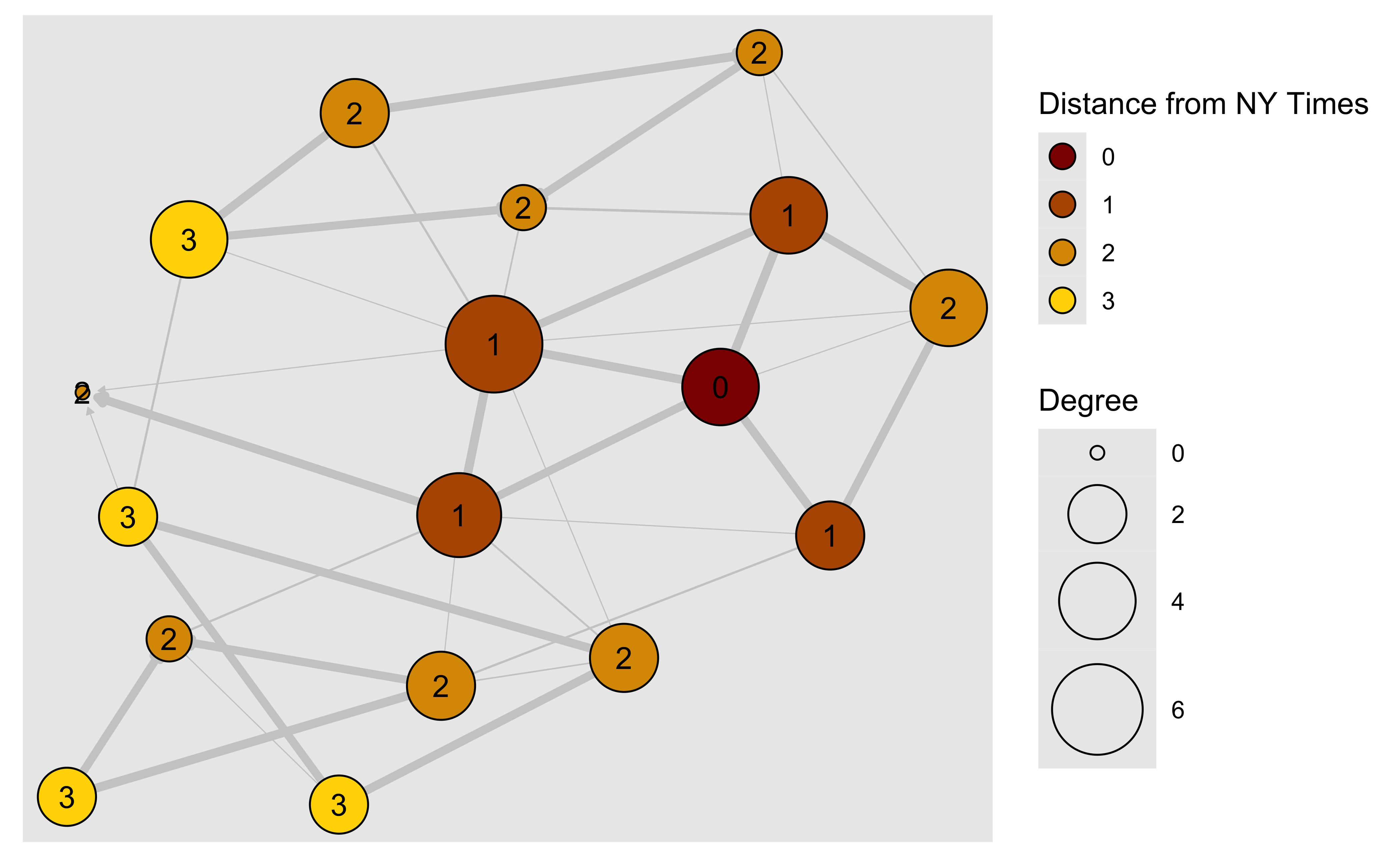
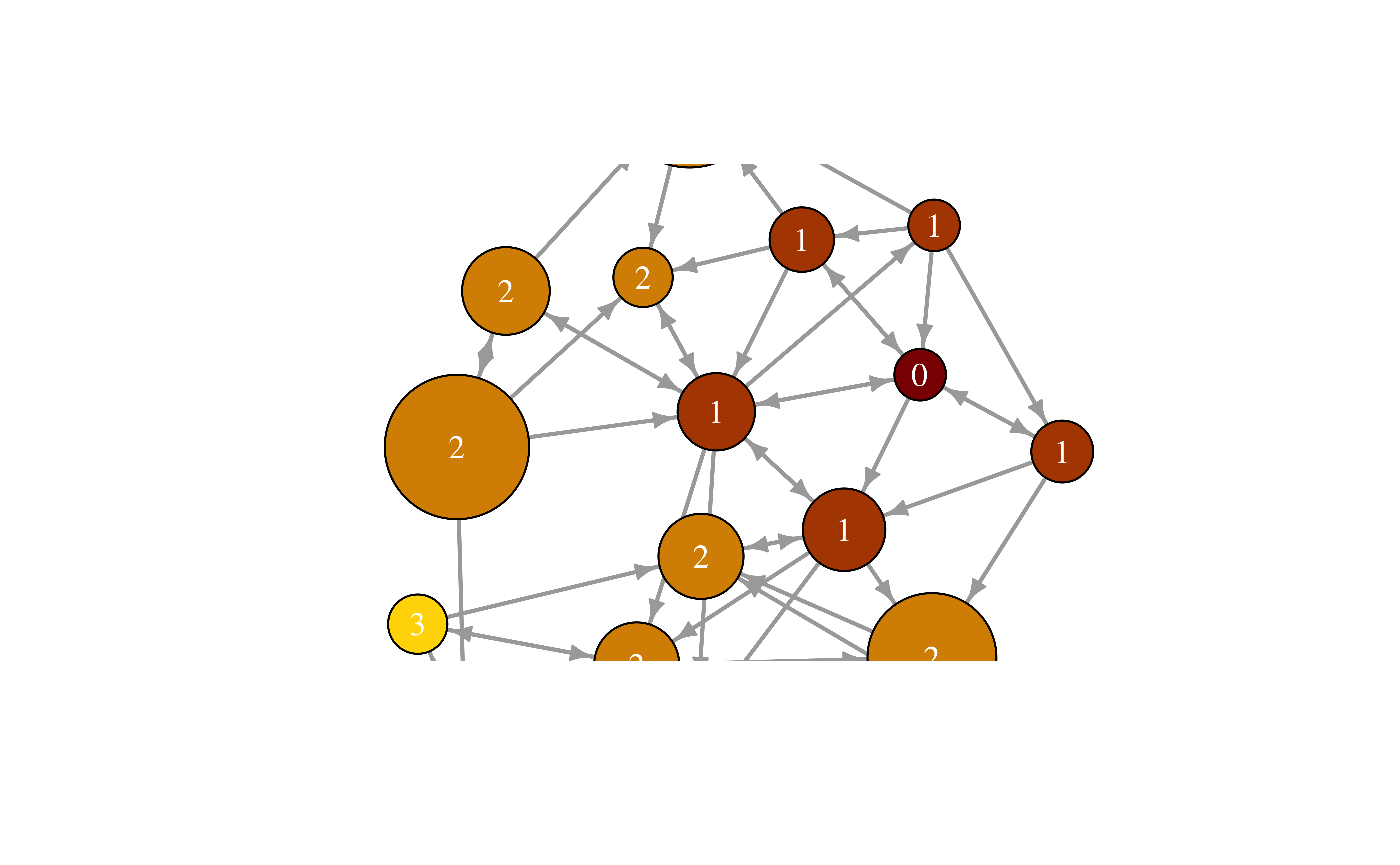
Sometimes we want to focus the visualization on a particular node or a group of nodes. Let’s represent distance from the NYT:

distances() calculates shortest path from vertices in ‘v’ to ones in ‘to’.

dist.from.NYT <- distances(net,
  v = V(net)[media == "NY Times"],
  to = V(net),
  weights = NA
)

# Set colors to plot the distances:
oranges <- colorRampPalette(c("dark red", "gold"))
col <- oranges(max(dist.from.NYT) + 1)
col <- col[dist.from.NYT + 1]

# Let's have same coordinates for Nodes in both graph renderings
# Then we can verify that the distance calculations are the same for both renderings
coords <- igraph::layout_nicely(net)
plot(net,
  vertex.label = dist.from.NYT,
  vertex.color = col, vertex.label.color = "black",
  layout = coords
)

# Using tidygraph
graph <- tbl_graph(nodes, links, directed = TRUE)
graph

# A tbl_graph: 17 nodes and 49 edges
#
# A directed multigraph with 1 component
#
# Node Data: 17 × 5 (active)
   id    media               media.type type.label audience.size
   <chr> <chr>                    <int> <chr>              <int>
 1 s01   NY Times                     1 Newspaper             20
 2 s02   Washington Post              1 Newspaper             25
 3 s03   Wall Street Journal          1 Newspaper             30
 4 s04   USA Today                    1 Newspaper             32
 5 s05   LA Times                     1 Newspaper             20
 6 s06   New York Post                1 Newspaper             50
 7 s07   CNN                          2 TV                    56
 8 s08   MSNBC                        2 TV                    34
 9 s09   FOX News                     2 TV                    60
10 s10   ABC                          2 TV                    23
11 s11   BBC                          2 TV                    34
12 s12   Yahoo News                   3 Online                33
13 s13   Google News                  3 Online                23
14 s14   Reuters.com                  3 Online                12
15 s15   NYTimes.com                  3 Online                24
16 s16   WashingtonPost.com           3 Online                28
17 s17   AOL.com                      3 Online                33
#
# Edge Data: 49 × 4
   from    to type      weight
  <int> <int> <chr>      <int>
1     1     2 hyperlink     22
2     1     3 hyperlink     22
3     1     4 hyperlink     21
# ℹ 46 more rows

# Set up NY Times as root node first
# V(net)[media == "NY Times"] cannot be used since it returns an `igraph.vs` ( i.e. a list ) object.
# We need an integer node id.
root_nyt <- graph %>%
  activate(nodes) %>%
  as_tibble() %>%
  rowid_to_column(var = "node_id") %>%
  filter(media == "NY Times") %>%
  select(node_id) %>%
  as_vector()
root_nyt

node_id 
      1

graph %>%
  activate(nodes) %>%
  mutate(size = centrality_degree()) %>%
  # new stuff:
  # breadth first search for all distances from the root node
  mutate(order = bfs_dist(root = root_nyt)) %>%
  ggraph(., layout = coords) + # same layout
  geom_edge_link(
    aes(width = weight),
    color = "grey80",
    end_cap = circle(.2, "cm"),
    arrow = arrow(
      type = "closed",
      ends = "last",
      length = unit(1, "mm")
    )
  ) +
  geom_node_point(
    aes(
      fill = order,
      size = size
    ),
    shape = 21,
    color = "black"
  ) +

  geom_node_text(aes(label = order)) +

  scale_fill_gradient(
    name = "Distance from NY Times",
    low = "dark red",
    high = "gold",
    guide = "legend"
  ) +
  scale_edge_width(range = c(0.2, 1.5), guide = "none") +
  scale_size_continuous("Degree", range = c(2, 16)) +
  guides(fill = guide_legend(override.aes = list(
    pch = 21,
    size = 4
  )))

Or, a bit more readable:

plot(net,
  vertex.color = col,
  vertex.label = dist.from.NYT, edge.arrow.size = .6,
  vertex.label.color = "white",
  vertex.size = V(net)$size * 1.6,
  edge.width = 2,
  layout = norm_coords(layout_with_lgl(net)) * 1.4, rescale = F
)

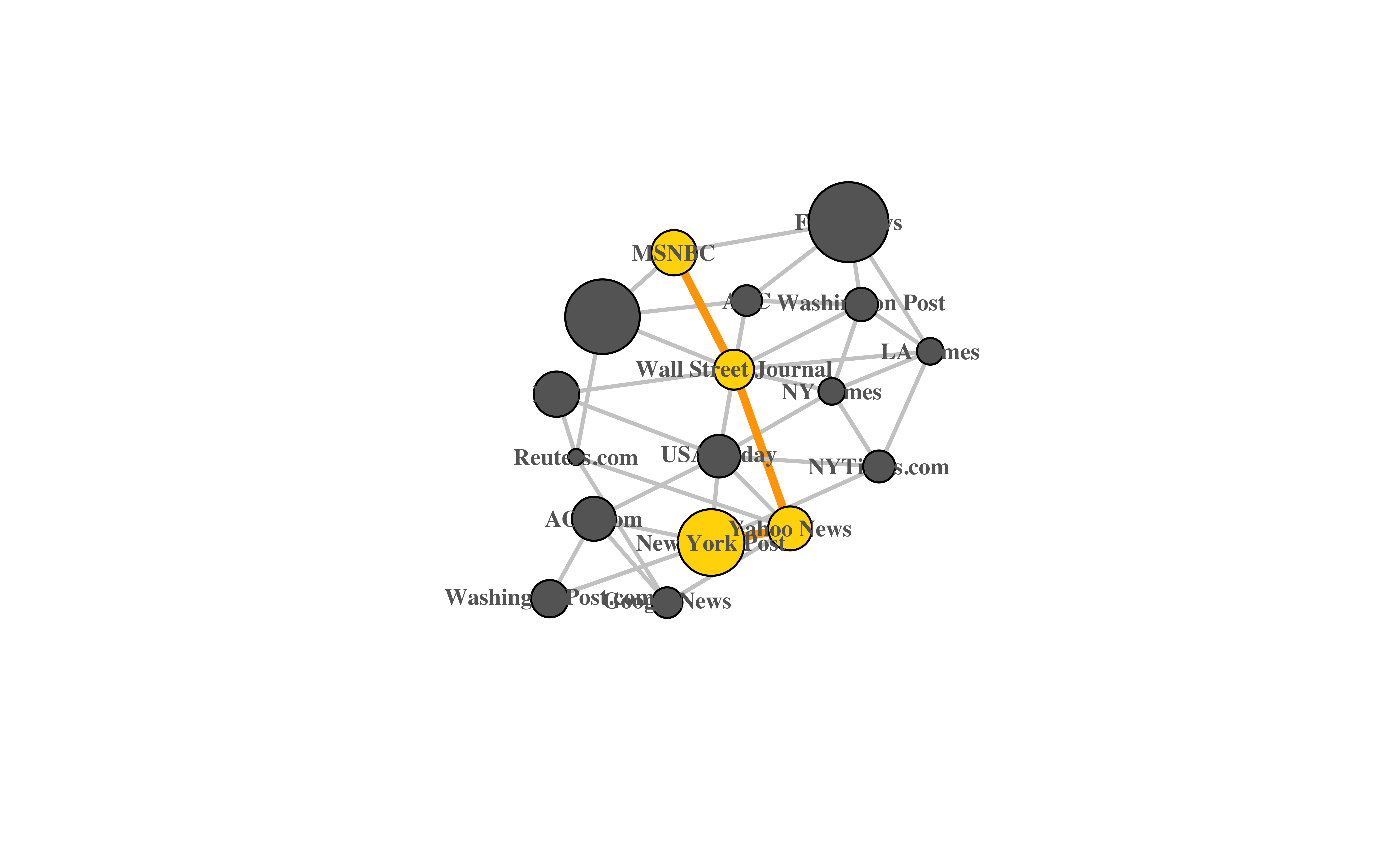
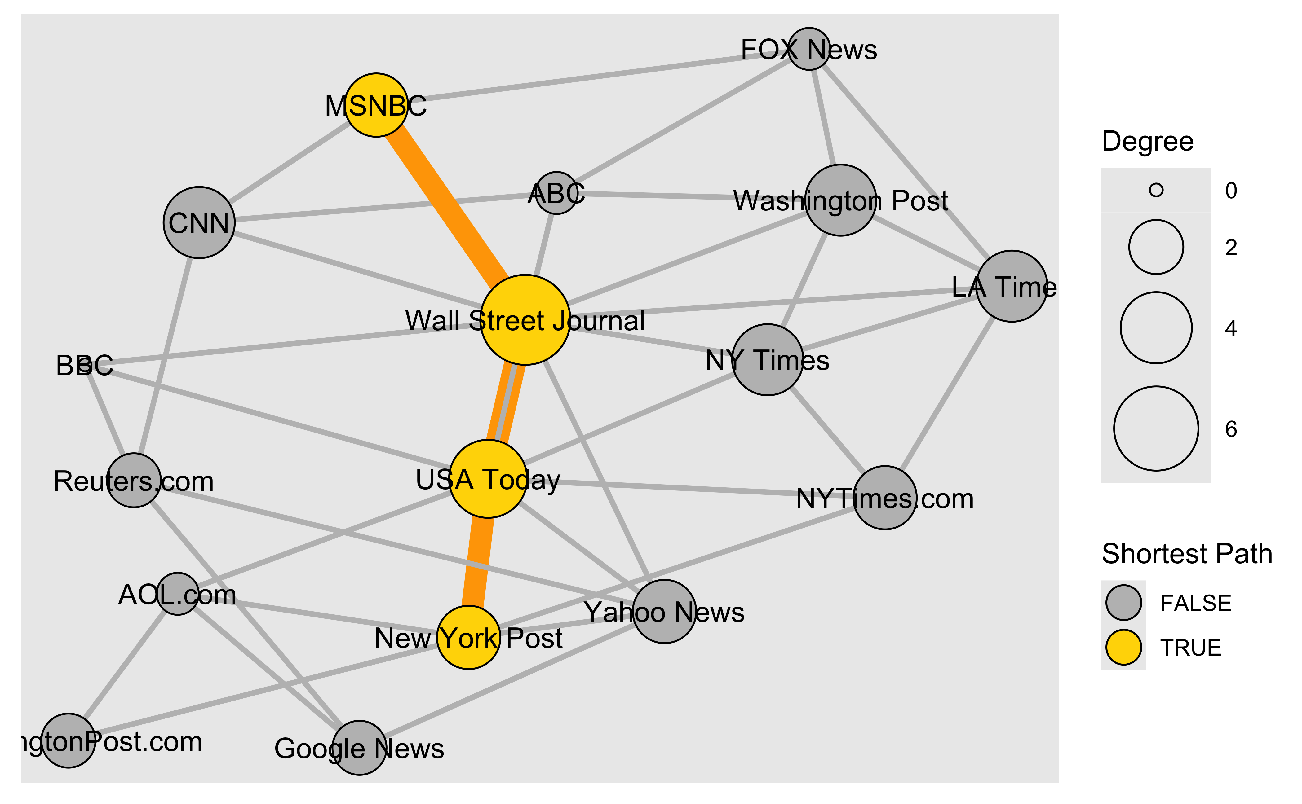
Path Highlighting

We can also highlight paths between the nodes in the network.

Say here between MSNBC and the New York Post

news.path <- shortest_paths(net,
  from = V(net)[media == "MSNBC"],
  to = V(net)[media == "New York Post"],
  output = "both"
) # both path nodes and edges
news.path.distance <- distances(
  net,
  V(net)[media == "MSNBC"],
  V(net)[media == "New York Post"]
)
news.path

$vpath
$vpath[[1]]
+ 4/17 vertices, named, from a98c0d8:
[1] s08 s03 s12 s06


$epath
$epath[[1]]
+ 3/48 edges from a98c0d8 (vertex names):
[1] s08->s03 s03->s12 s12->s06


$predecessors
NULL

$inbound_edges
NULL

news.path.distance

    s06
s08   5

# Generate edge color variable to plot the path:
ecol <- rep("gray80", ecount(net))
ecol[unlist(news.path$epath)] <- "orange"

# Generate edge width variable to plot the path:
ew <- rep(2, ecount(net))
ew[unlist(news.path$epath)] <- 4

# Generate node color variable to plot the path:
vcol <- rep("gray40", vcount(net))
vcol[unlist(news.path$vpath)] <- "gold"

plot(net,
  vertex.color = vcol,
  edge.color = ecol,
  edge.width = ew,
  edge.arrow.mode = 0,
  ## added lines
  vertex.label = V(net)$media,
  vertex.label.font = 2,
  vertex.label.color = "gray40",
  vertex.label.cex = .7,
  layout = coords * 1.5
)

# Using tidygraph
# We need to use:
# to_shortest_path(graph, from, to, mode = "out", weights = NULL)
# Let's set up `to` and `from` nodes
#
# V(net)[media == "NY Times"] cannot be used since it returns an `igraph.vs` ( i.e. a list ) object.
# We need integer node ids for `from` and `to` in `to_shortest_path`

msnbc <- graph %>%
  activate(nodes) %>%
  as_tibble() %>%
  rowid_to_column(var = "node_id") %>%
  filter(media == "MSNBC") %>%
  select(node_id) %>%
  as_vector()
msnbc

node_id 
      8

nypost <- graph %>%
  activate(nodes) %>%
  as_tibble() %>%
  rowid_to_column(var = "node_id") %>%
  filter(media == "New York Post") %>%
  select(node_id) %>%
  as_vector()
nypost

node_id 
      6

# Let's create a fresh graph object using morph
# However we want to merge it back with the original `graph`
# to get an overlay plot
#
# # Can do this to obtain a separate graph
# convert(to_shortest_path,from = msnbc,to = nypost)
# However we want to merge it back with the original `graph`
# to get an overlay plot
msnbc_nyp <-
  graph %>%
  # first mark all nodes and edges as *not* on the shortest path
  activate(nodes) %>%
  mutate(shortest_path_node = FALSE) %>%
  activate(edges) %>%
  mutate(shortest_path_edge = FALSE) %>%
  # Find shortest path between MSNBC and NY Post
  morph(to_shortest_path, from = msnbc, to = nypost) %>%
  # Now to mark the shortest_path nodes as TRUE
  activate(nodes) %>%
  mutate(shortest_path_node = TRUE) %>%
  # Now to mark the shortest_path edges as TRUE
  activate(edges) %>%
  mutate(shortest_path_edge = TRUE) %>%
  #
  # Merge back into main graph; Still saving it as a `msnbc_nyp`
  unmorph()
msnbc_nyp

# A tbl_graph: 17 nodes and 49 edges
#
# A directed multigraph with 1 component
#
# Edge Data: 49 × 5 (active)
    from    to type      weight shortest_path_edge
   <int> <int> <chr>      <int> <lgl>             
 1     1     2 hyperlink     22 FALSE             
 2     1     3 hyperlink     22 FALSE             
 3     1     4 hyperlink     21 FALSE             
 4     1    15 mention       20 FALSE             
 5     2     1 hyperlink     23 FALSE             
 6     2     3 hyperlink     21 FALSE             
 7     2     9 hyperlink      1 FALSE             
 8     2    10 hyperlink      5 FALSE             
 9     3     1 hyperlink     21 FALSE             
10     3     4 hyperlink     22 TRUE              
# ℹ 39 more rows
#
# Node Data: 17 × 6
  id    media             media.type type.label audience.size shortest_path_node
  <chr> <chr>                  <int> <chr>              <int> <lgl>             
1 s01   NY Times                   1 Newspaper             20 FALSE             
2 s02   Washington Post            1 Newspaper             25 FALSE             
3 s03   Wall Street Jour…          1 Newspaper             30 TRUE              
# ℹ 14 more rows

msnbc_nyp %>%
  activate(nodes) %>%
  mutate(size = centrality_degree()) %>%
  ggraph(layout = coords) +
  # geom_edge_link0(colour = "grey") +
  geom_edge_link0(aes(
    colour = shortest_path_edge,
    width = shortest_path_edge
  )) +

  geom_node_point(aes(
    size = size,
    fill = shortest_path_node
  ), shape = 21) +
  geom_node_text(aes(label = media)) +

  scale_size_continuous("Degree", range = c(2, 16)) +
  scale_fill_manual("Shortest Path",
    values = c("grey", "gold")
  ) +

  scale_edge_width_manual(values = c(1, 4)) +

  scale_edge_colour_manual(values = c("grey", "orange")) +
  guides(
    fill = guide_legend(override.aes = list(
      pch = 21,
      size = 6
    )),
    edge_colour = "none",
    edge_width = "none"
  )

Highlight the edges going into or out of a vertex, for instance the WSJ. For a single node, use incident(), for multiple nodes use incident_edges()

inc.edges <-
  incident(net, V(net)[media == "Wall Street Journal"], mode = "all")

# Set colors to plot the selected edges.
ecol <- rep("gray80", ecount(net))
ecol[inc.edges] <- "orange"
vcol <- rep("grey40", vcount(net))
vcol[V(net)$media == "Wall Street Journal"] <- "gold"
plot(
  net,
  vertex.color = vcol,
  edge.color = ecol,
  edge.width = 2,
  layout = coords
)

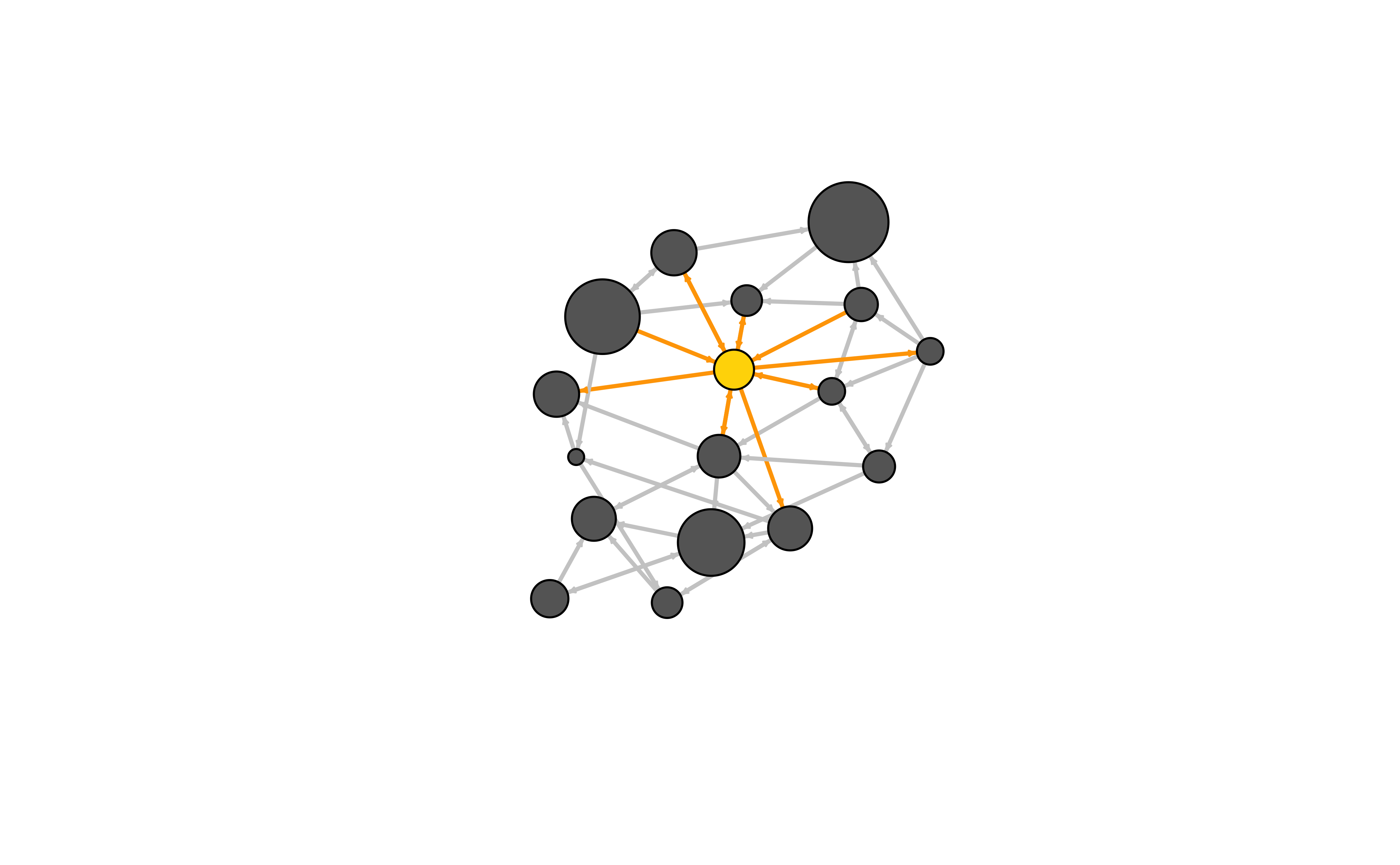
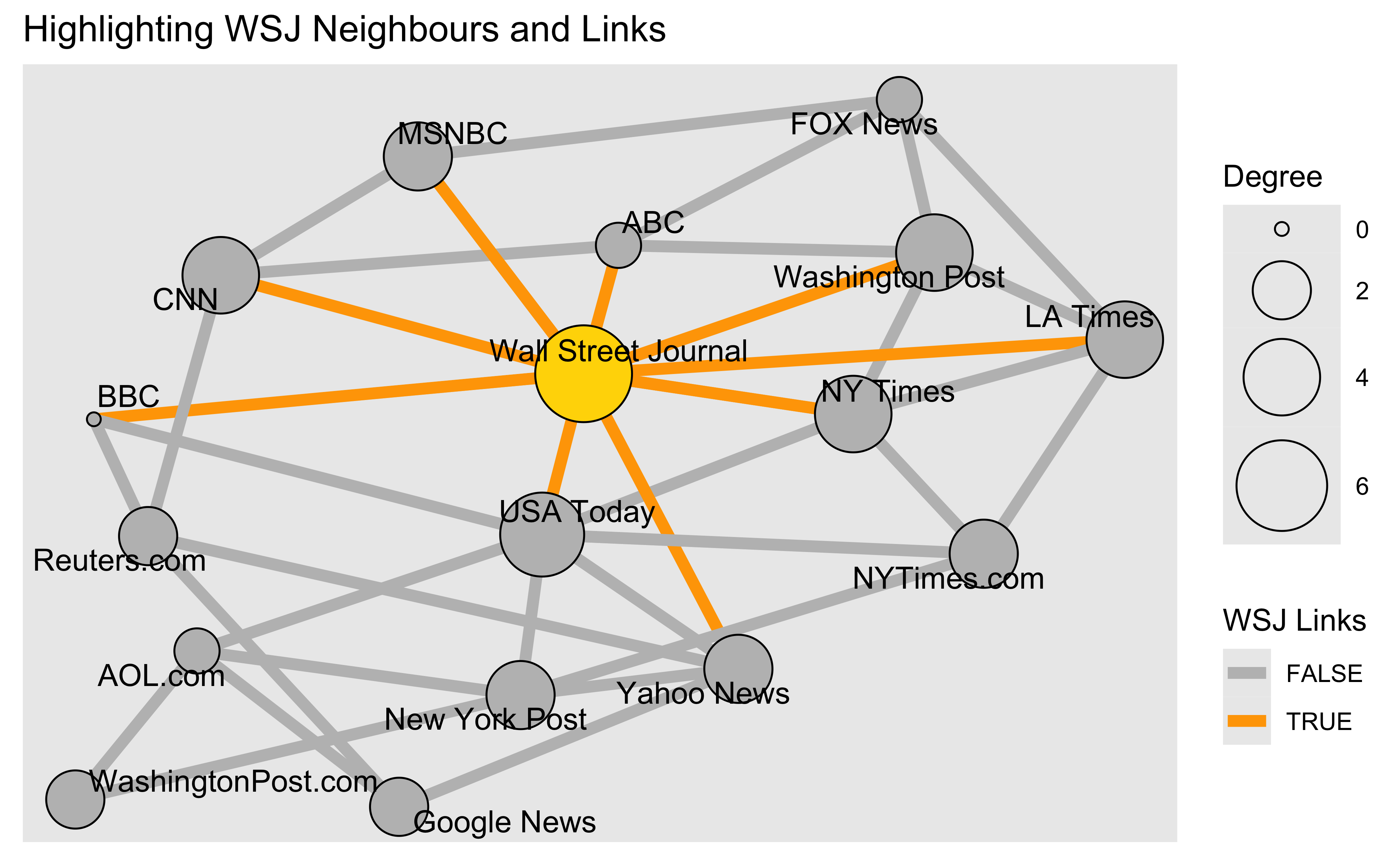
# Using tidygraph
wsj <- graph %>%
  activate(nodes) %>%
  as_tibble() %>%
  rowid_to_column(var = "node_id") %>%
  filter(media == "Wall Street Journal") %>%
  select(node_id) %>%
  as_vector()

graph %>%
  activate(nodes) %>%
  mutate(
    wsj_adjacent = node_is_adjacent(
      to = wsj, mode = "all",
      include_to = TRUE
    ),
    size = centrality_degree()
  ) %>%
  mutate(WSJ = if_else(media == "Wall Street Journal", TRUE, FALSE)) %>%
  activate(edges) %>%
  mutate(wsj_links = edge_is_incident(wsj)) %>%
  ggraph(., layout = coords) +
  geom_edge_link0(aes(colour = wsj_links), width = 2) +

  geom_node_point(aes(
    fill = WSJ,
    size = size
  ), shape = 21) +

  geom_node_text(aes(label = media), repel = TRUE) +

  scale_fill_manual("WSJ Neighbours",
    values = c("grey", "gold"),
    guide = guide_legend(
      override.aes =
        list(
          pch = 21,
          size = 5
        )
    )
  ) +
  scale_edge_colour_manual("WSJ Links",
    values = c("grey", "orange")
  ) +
  scale_size("Degree", range = c(2, 16)) +
  ggtitle(label = "Highlighting WSJ Neighbours and Links") +
  guides(
    shape = "none", fill = "none" # , colour = "none"
  )

Highlight Neighbours

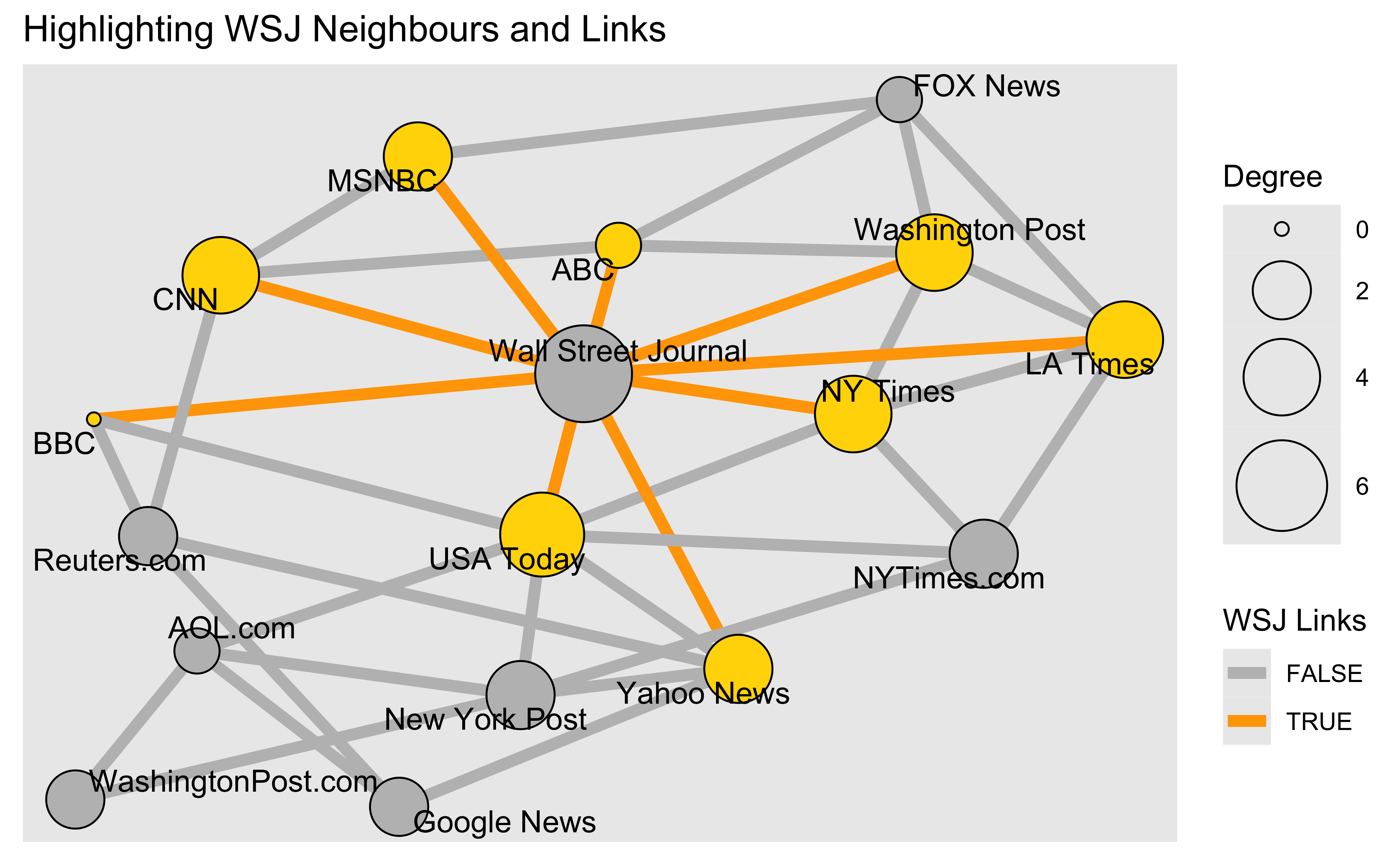
Or we can highlight the immediate neighbors of a vertex, say WSJ. The neighbors function finds all nodes one step out from the focal actor. To find the neighbors for multiple nodes, use adjacent_vertices(). To find node neighborhoods going more than one step out, use function ego() with parameter order set to the number of steps out to go from the focal node(s).

neigh.nodes <- neighbors(net, V(net)[media == "Wall Street Journal"], mode = "out")

# Set colors to plot the neighbors:
vcol[neigh.nodes] <- "#ff9d00"
plot(net, vertex.color = vcol)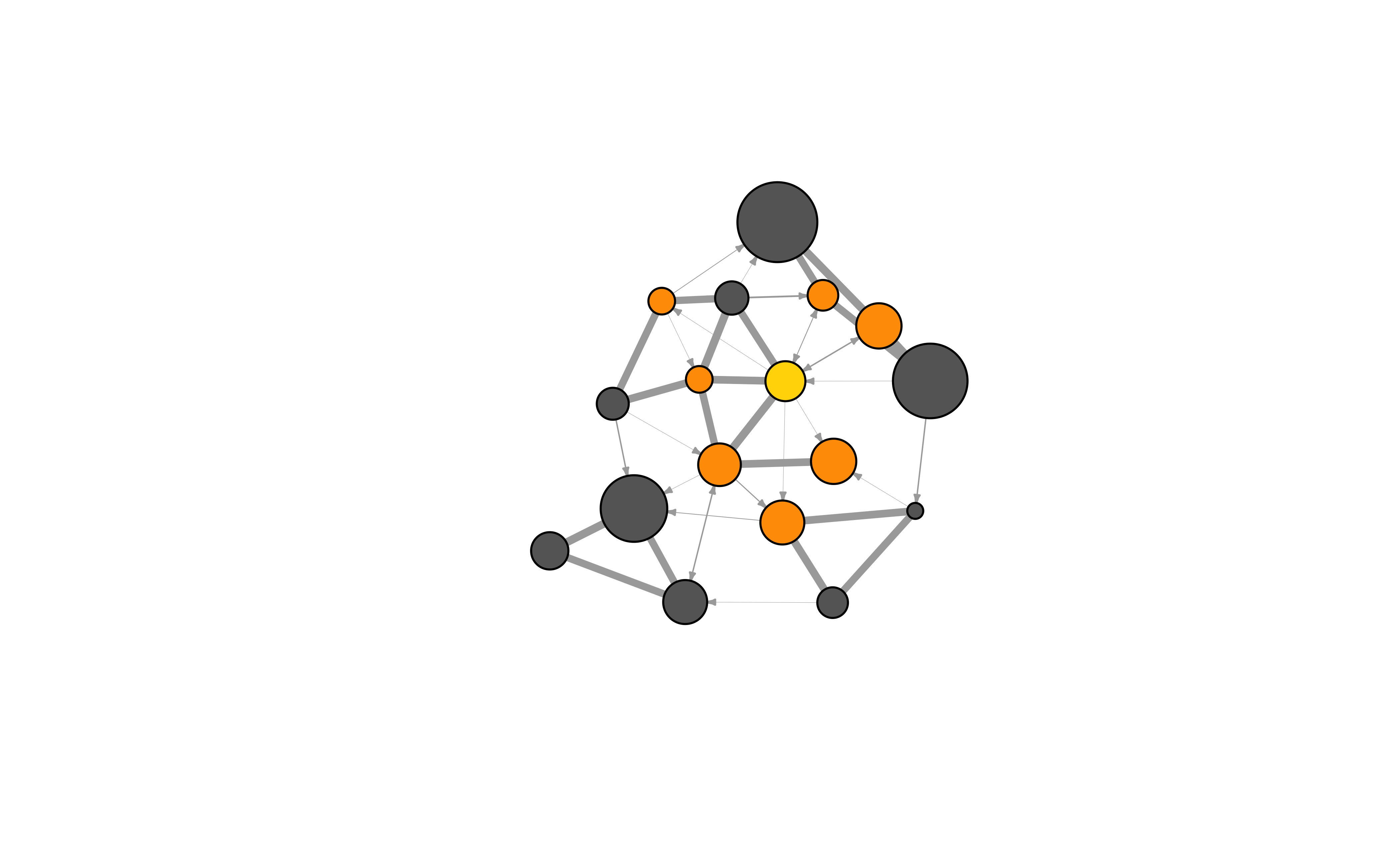

# Using tidygraph
wsj <- graph %>%
  activate(nodes) %>%
  as_tibble() %>%
  rowid_to_column(var = "node_id") %>%
  filter(media == "Wall Street Journal") %>%
  select(node_id) %>%
  as_vector()

graph %>%
  activate(nodes) %>%
  mutate(
    wsj_adjacent = node_is_adjacent(
      to = wsj, mode = "all",
      # remove WSJ from the list!
      # highlight only the neighbours

      include_to = FALSE
    ),
    size = centrality_degree()
  ) %>%
  mutate(WSJ = if_else(media == "Wall Street Journal", TRUE, FALSE)) %>%
  activate(edges) %>%
  mutate(wsj_links = edge_is_incident(wsj)) %>%
  ggraph(., layout = coords) +
  geom_edge_link0(aes(colour = wsj_links), width = 2) +

  geom_node_point(aes(
    fill = wsj_adjacent,
    size = size
  ), shape = 21) +

  geom_node_text(aes(label = media), repel = TRUE) +

  scale_fill_manual("WSJ Neighbours",
    values = c("grey", "gold"),
    guide = guide_legend(
      override.aes =
        list(
          pch = 21,
          size = 5
        )
    )
  ) +
  scale_edge_colour_manual("WSJ Links",
    values = c("grey", "orange")
  ) +
  scale_size("Degree", range = c(2, 16)) +
  ggtitle(label = "Highlighting WSJ Neighbours and Links") +
  guides(
    shape = "none", fill = "none" # , colour = "none"
  )

Another way to draw attention to a group of nodes: (This is generally not recommended since, depending on layout, nodes that are not ‘marked’ can accidentally get placed on top of the mark)

plot(net, mark.groups = c(1, 4, 5, 8), mark.col = "#C5E5E7", mark.border = NA)

# Mark multiple groups:
plot(net,
  mark.groups = list(c(1, 4, 5, 8), c(15:17)),
  mark.col = c("#C5E5E7", "#ECD89A"), mark.border = NA
)

——-~~ Interactive plotting with ‘tkplot’ ——–

R and igraph offer interactive plotting capabilities (mostly helpful for small networks)

tkid <- tkplot(net) # tkid is the id of the tkplot

l <- tkplot.getcoords(tkid) # grab the coordinates from tkplot
plot(net, layout = l)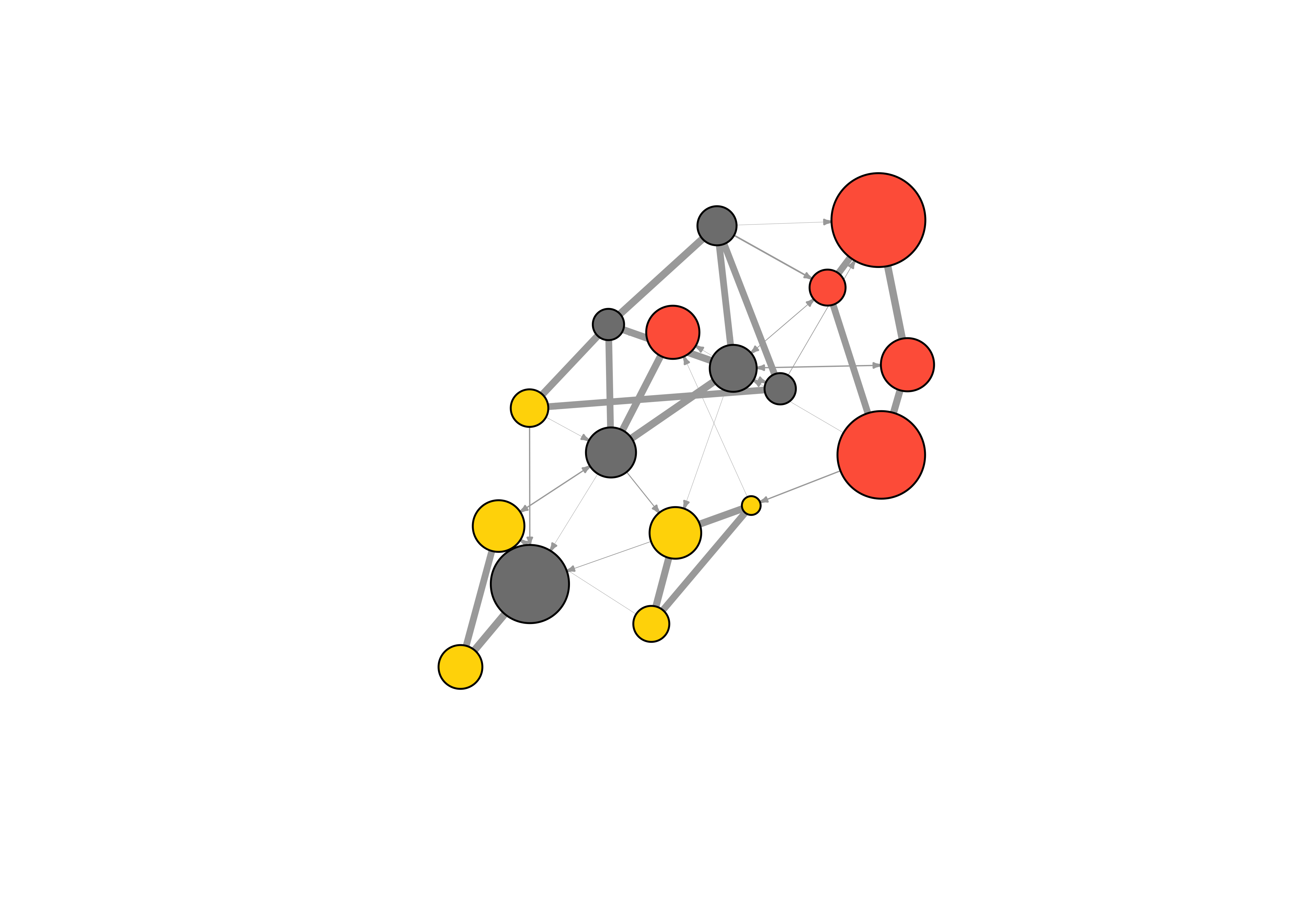

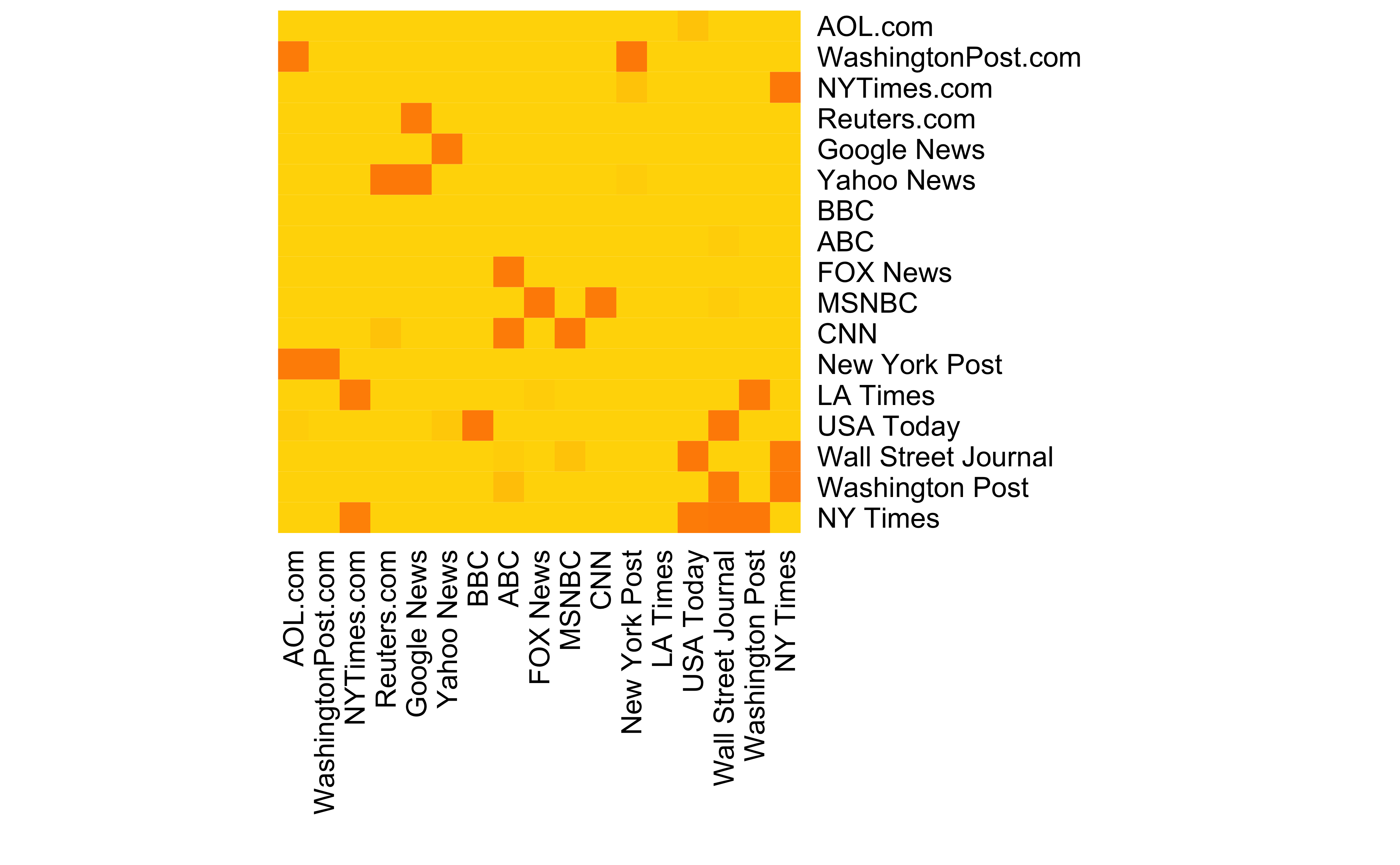
——-~~ Other ways to represent a network ——–

One reminder that there are other ways to represent a network:

Heatmap of the network matrix:

netm <- as_adjacency_matrix(net, attr = "weight", sparse = F)
colnames(netm) <- V(net)$media
rownames(netm) <- V(net)$media

palf <- colorRampPalette(c("gold", "dark orange"))

# The Rowv & Colv parameters turn dendrograms on and off
heatmap(netm[, 17:1],
  Rowv = NA, Colv = NA, col = palf(20),
  scale = "none", margins = c(10, 10)
)

Degree distribution

deg.dist <- degree_distribution(net, cumulative = T, mode = "all")
# degree is available in `sna` too
plot(x = 0:max(igraph::degree(net)), y = 1 - deg.dist, pch = 19, cex = 1.4, col = "orange", xlab = "Degree", ylab = "Cumulative Frequency")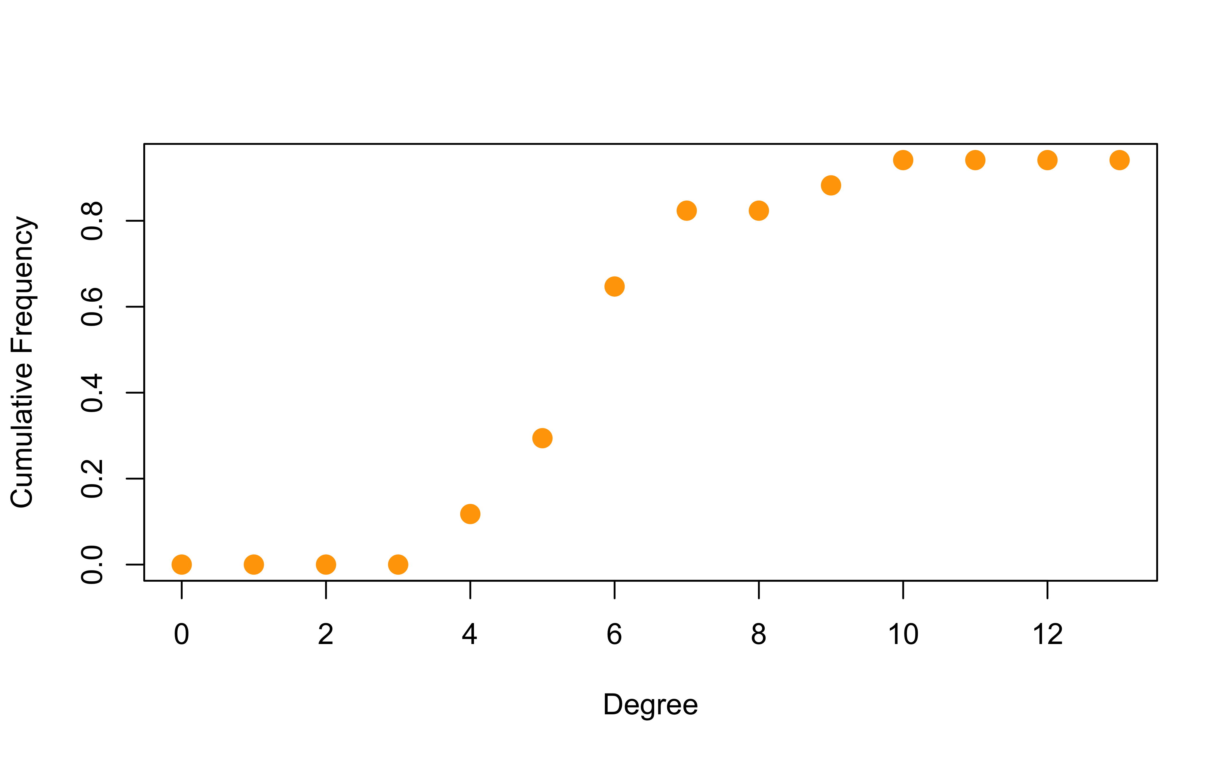

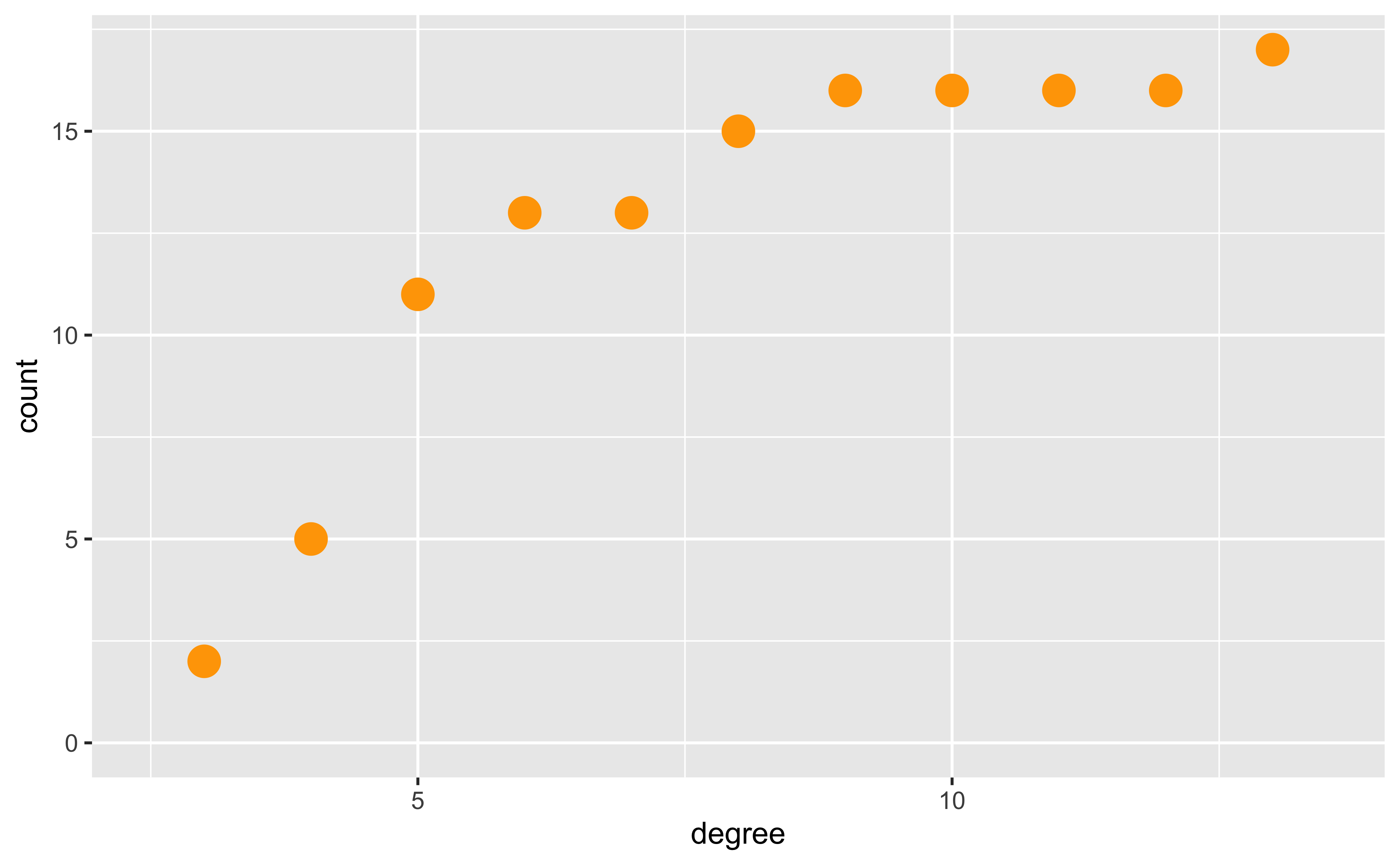
# Using Tidygraph
# https://stackoverflow.com/questions/18356860/cumulative-histogram-with-ggplot2
graph %>%
  activate(nodes) %>%
  mutate(degree = centrality_degree(mode = "all")) %>%
  as_tibble() %>%
  ggplot(aes(x = degree, y = stat(count))) +
  # geom_histogram(aes(y = cumsum(..count..)), binwidth = 1) +
  stat_bin(aes(y = cumsum(after_stat(count))),
    binwidth = 1, # Ta-Da !!
    geom = "point", color = "orange", size = 5
  )

4. Plotting two-mode networks

head(nodes2)

ABCDEFGHIJ0123456789

	id <chr>	media <chr>	media.type <int>	media.name <chr>	audience.size <int>
1	s01	NYT	1	Newspaper	20
2	s02	WaPo	1	Newspaper	25
3	s03	WSJ	1	Newspaper	30
4	s04	USAT	1	Newspaper	32
5	s05	LATimes	1	Newspaper	20
6	s06	CNN	2	TV	56

head(links2)

    U01 U02 U03 U04 U05 U06 U07 U08 U09 U10 U11 U12 U13 U14 U15 U16 U17 U18 U19
s01   1   1   1   0   0   0   0   0   0   0   0   0   0   0   0   0   0   0   0
s02   0   0   0   1   1   0   0   0   0   0   0   0   0   0   0   0   0   0   0
s03   0   0   0   0   0   1   1   1   1   0   0   0   0   0   0   0   0   0   0
s04   0   0   0   0   0   0   0   0   1   1   1   0   0   0   0   0   0   0   0
s05   0   0   0   0   0   0   0   0   0   0   1   1   1   0   0   0   0   0   0
s06   0   0   0   0   0   0   0   0   0   0   0   0   1   1   0   0   1   0   0
    U20
s01   0
s02   1
s03   0
s04   0
s05   0
s06   0

net2

IGRAPH 330c2c6 UN-B 30 31 -- 
+ attr: type (v/l), name (v/c)
+ edges from 330c2c6 (vertex names):
 [1] s01--U01 s01--U02 s01--U03 s02--U04 s02--U05 s02--U20 s03--U06 s03--U07
 [9] s03--U08 s03--U09 s04--U09 s04--U10 s04--U11 s05--U11 s05--U12 s05--U13
[17] s06--U13 s06--U14 s06--U17 s07--U14 s07--U15 s07--U16 s08--U16 s08--U17
[25] s08--U18 s08--U19 s09--U06 s09--U19 s09--U20 s10--U01 s10--U11

plot(net2)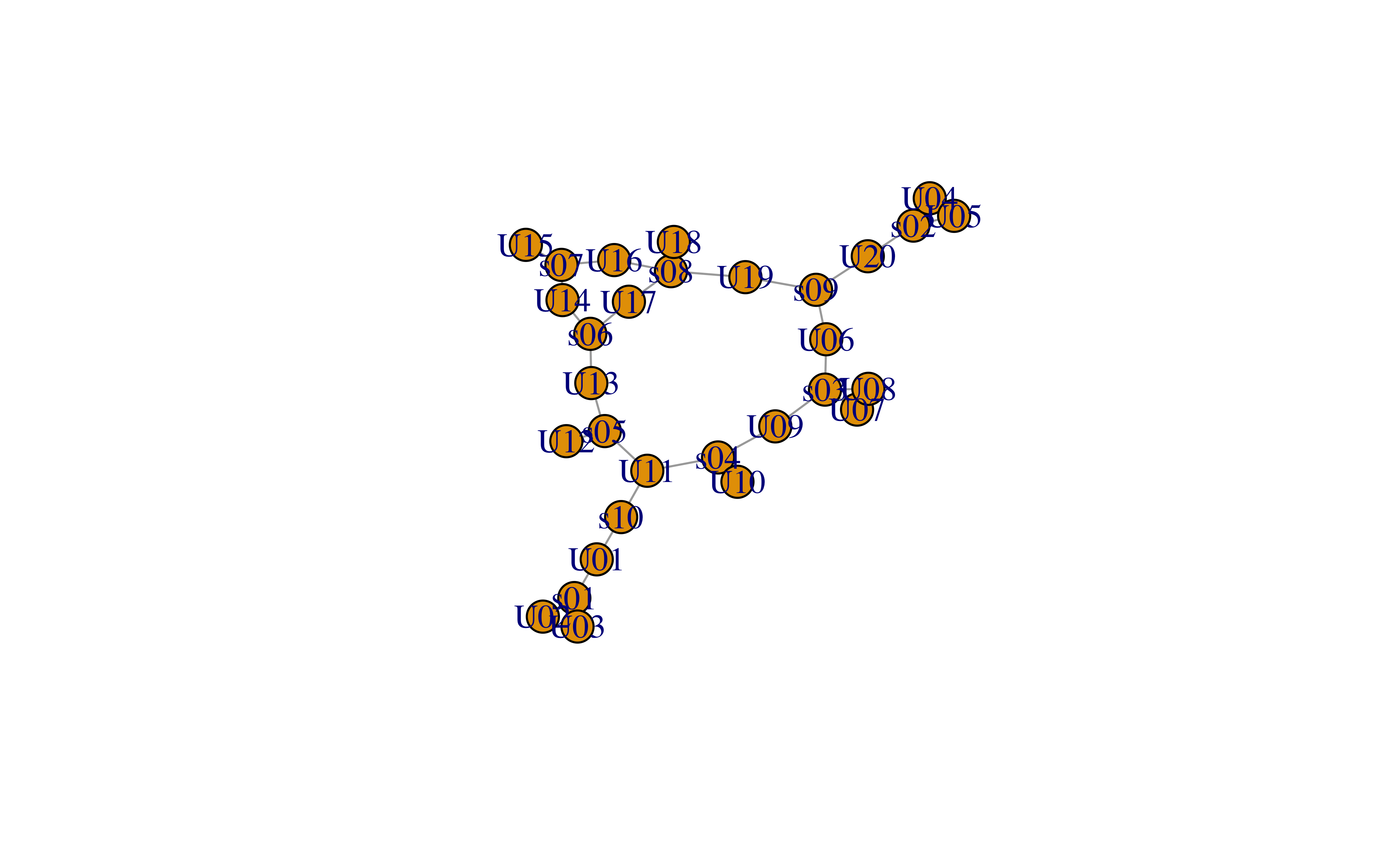

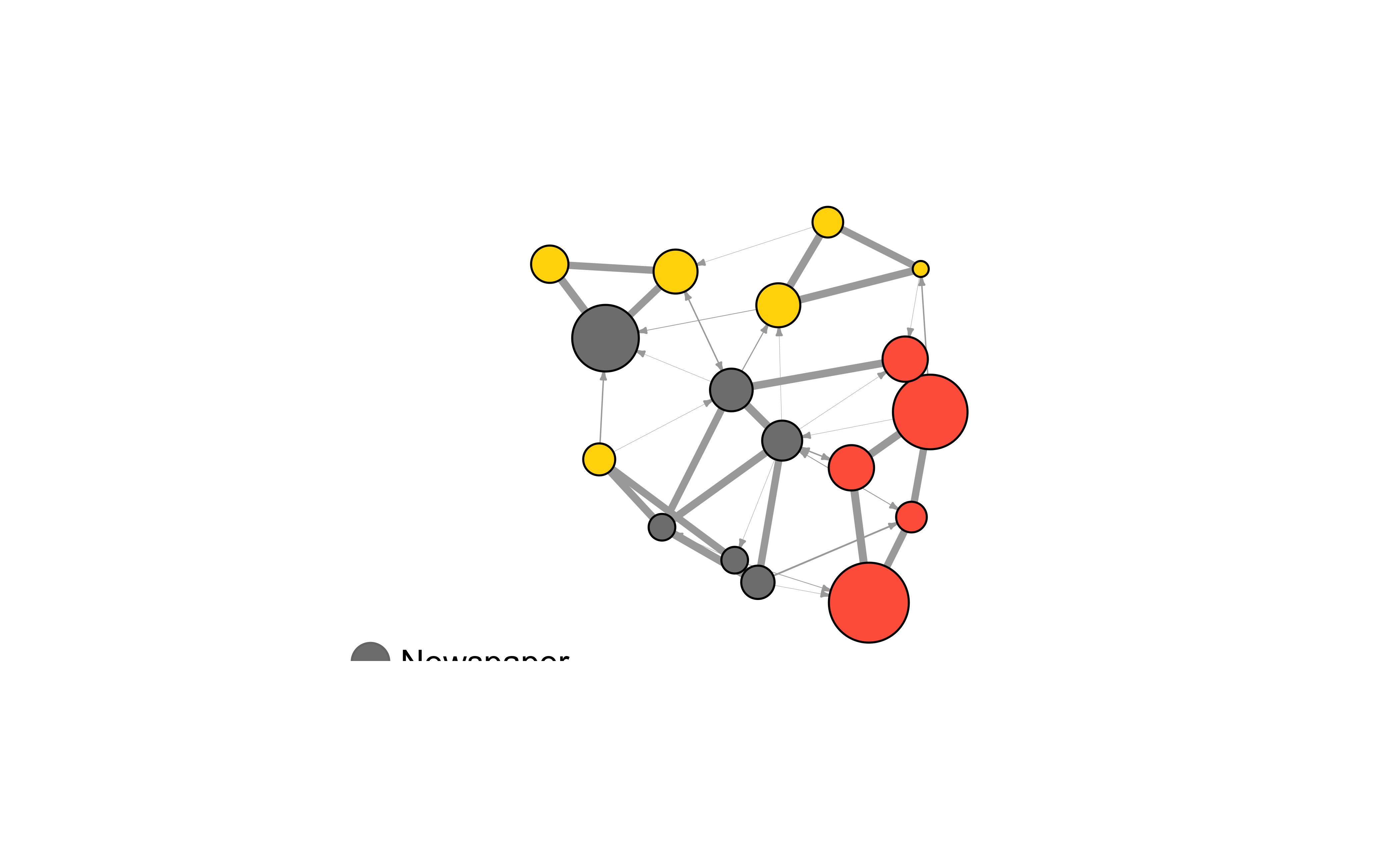
This time we will make nodes look different based on their type. Media outlets are blue squares, audience nodes are orange circles:

V(net2)$color <- c("steel blue", "orange")[V(net2)$type + 1]
V(net2)$shape <- c("square", "circle")[V(net2)$type + 1]

# Media outlets will have name labels, audience members will not:
V(net2)$label <- ""
V(net2)$label[V(net2)$type == F] <- nodes2$media[V(net2)$type == F]
V(net2)$label.cex <- .6
V(net2)$label.font <- 2

plot(net2, vertex.label.color = "white", vertex.size = (2 - V(net2)$type) * 8)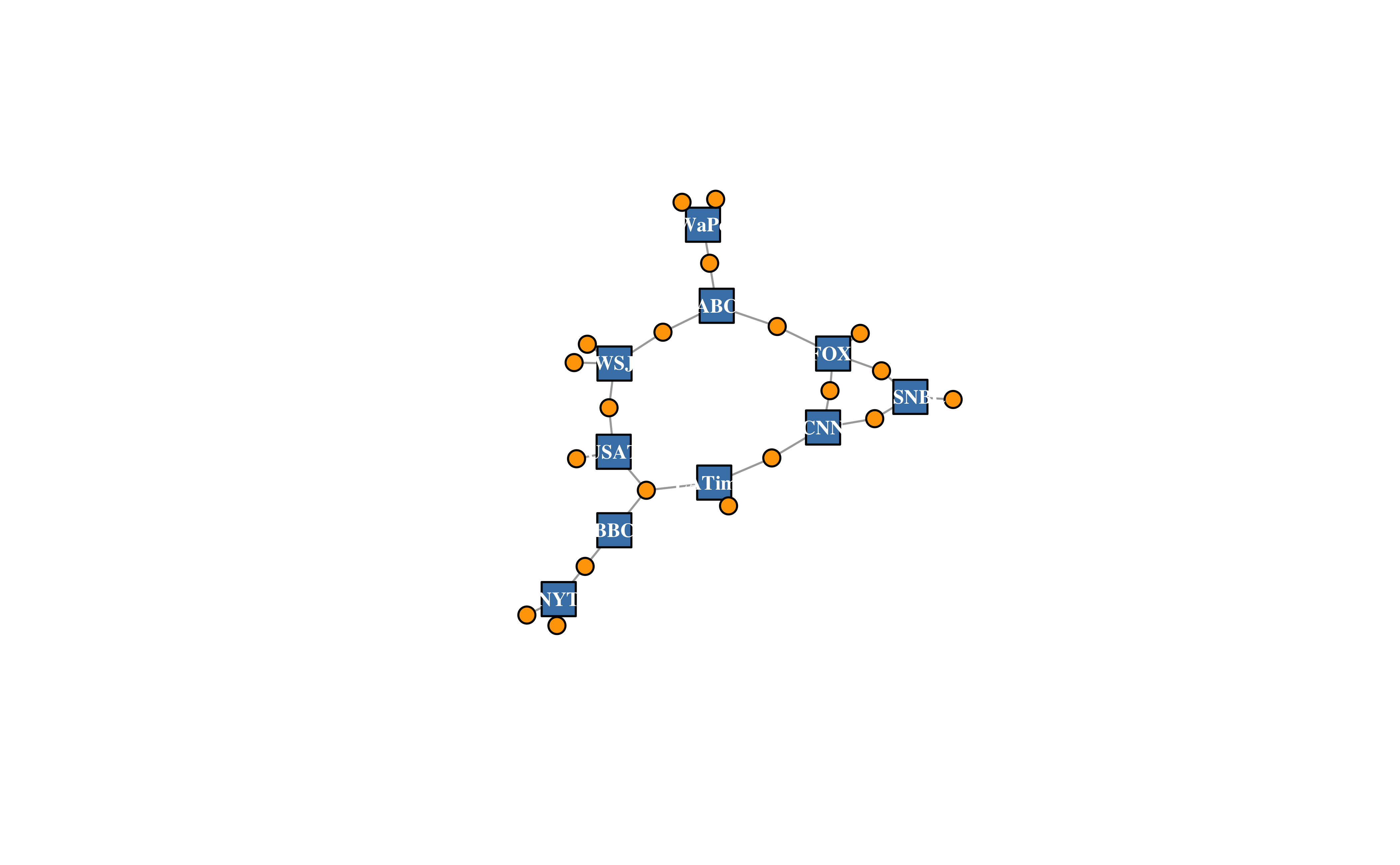

# Using tidygraph
as_tbl_graph(x = links2, directed = TRUE) %>%
  activate(nodes) %>%
  left_join(nodes2, by = c("name" = "id")) %>%
  ggraph(layout = "nicely") +
  geom_edge_link0() +
  geom_node_point(aes(shape = type, fill = type, size = type)) +
  geom_node_text(aes(label = if_else(type, "", media)), colour = "white", size = 3) +

  scale_shape_manual(
    "Type",
    values = c(22, 21),
    labels = c("Media", "Persons"),
    guide = guide_legend(override.aes = list(size = 6))
  ) +

  scale_fill_manual(
    "Type",
    values = c("dodgerblue", "orange"),
    labels = c("Media", "Persons")
  ) +

  scale_size_manual(values = c(10, 4), guide = "none")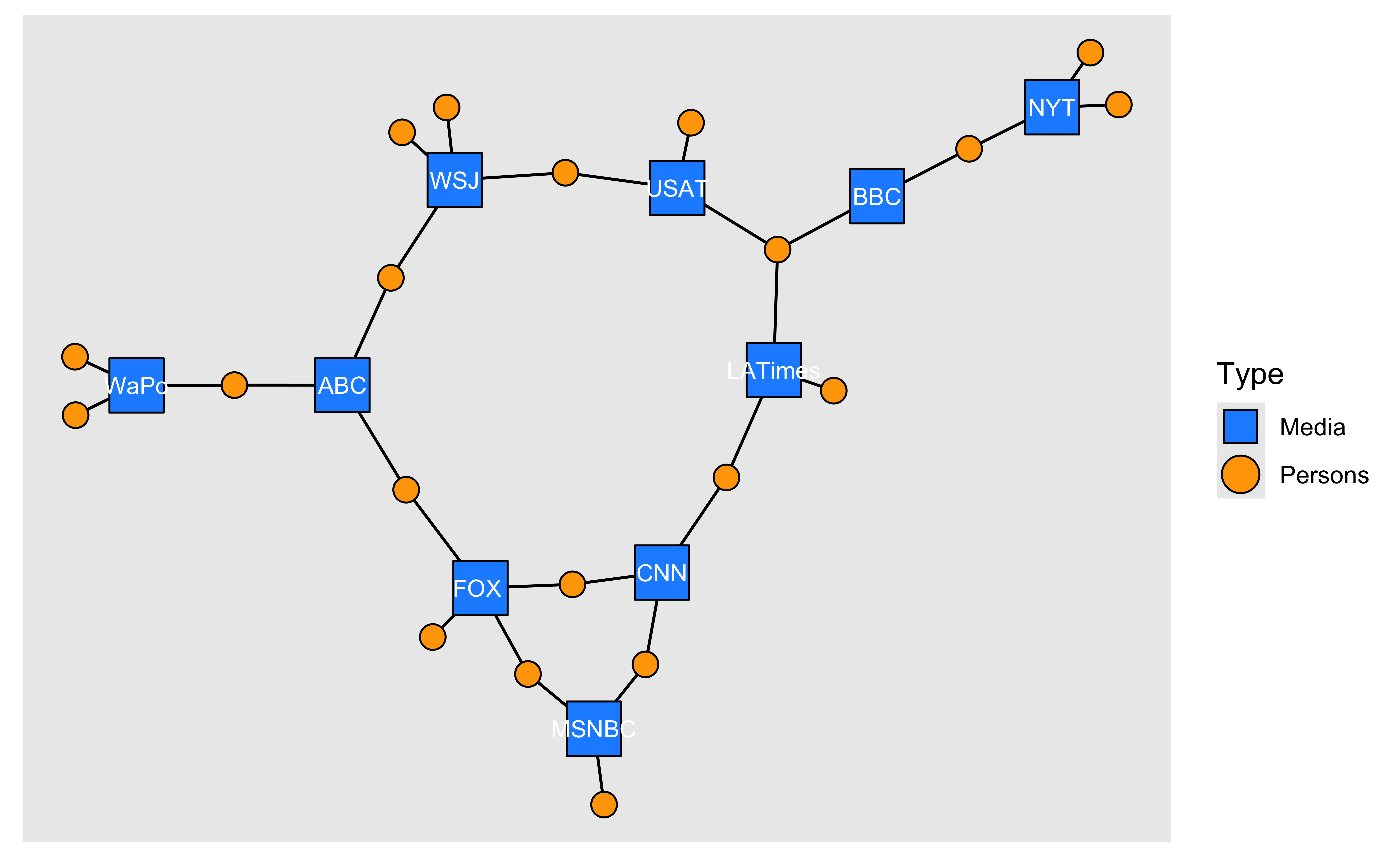

igraph has a built-in bipartite layout, though it’s not the most helpful:

plot(net2, vertex.label = NA, vertex.size = 7, layout = layout_as_bipartite)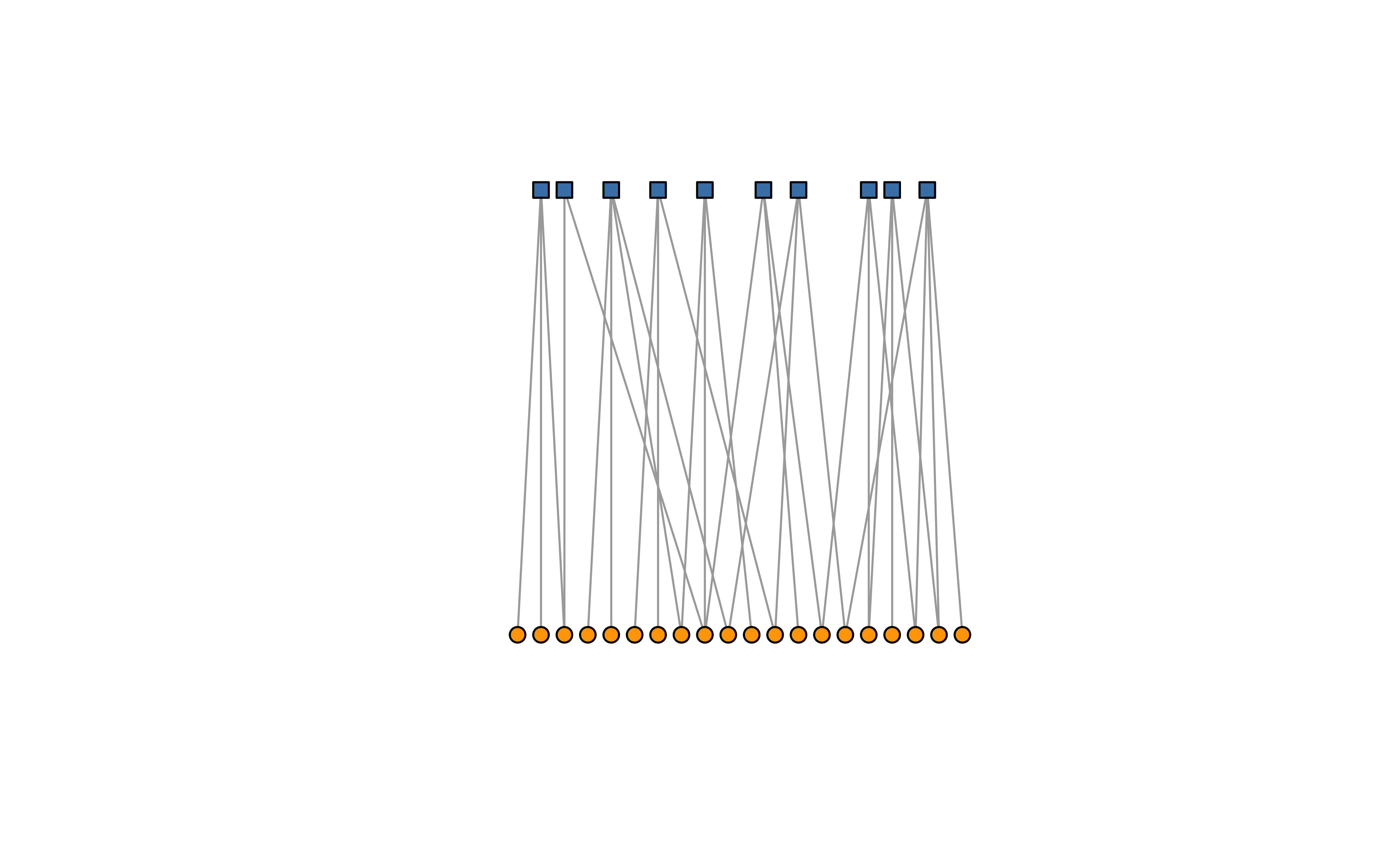

# using tidygraph
as_tbl_graph(x = links2, directed = TRUE) %>%
  activate(nodes) %>%
  left_join(nodes2, by = c("name" = "id")) %>%
  ggraph(., layout = "igraph", algorithm = "bipartite") +
  geom_edge_link0() +
  geom_node_point(aes(shape = type, fill = type, size = type)) +
  geom_node_text(aes(label = if_else(type, "", media)), colour = "white", size = 3) +

  scale_shape_manual(
    "Type",
    values = c(22, 21),
    labels = c("Media", "Persons"),
    guide = guide_legend(override.aes = list(size = 6))
  ) +

  scale_fill_manual(
    "Type",
    values = c("dodgerblue", "orange"),
    labels = c("Media", "Persons")
  ) +

  scale_size_manual(values = c(10, 4), guide = "none")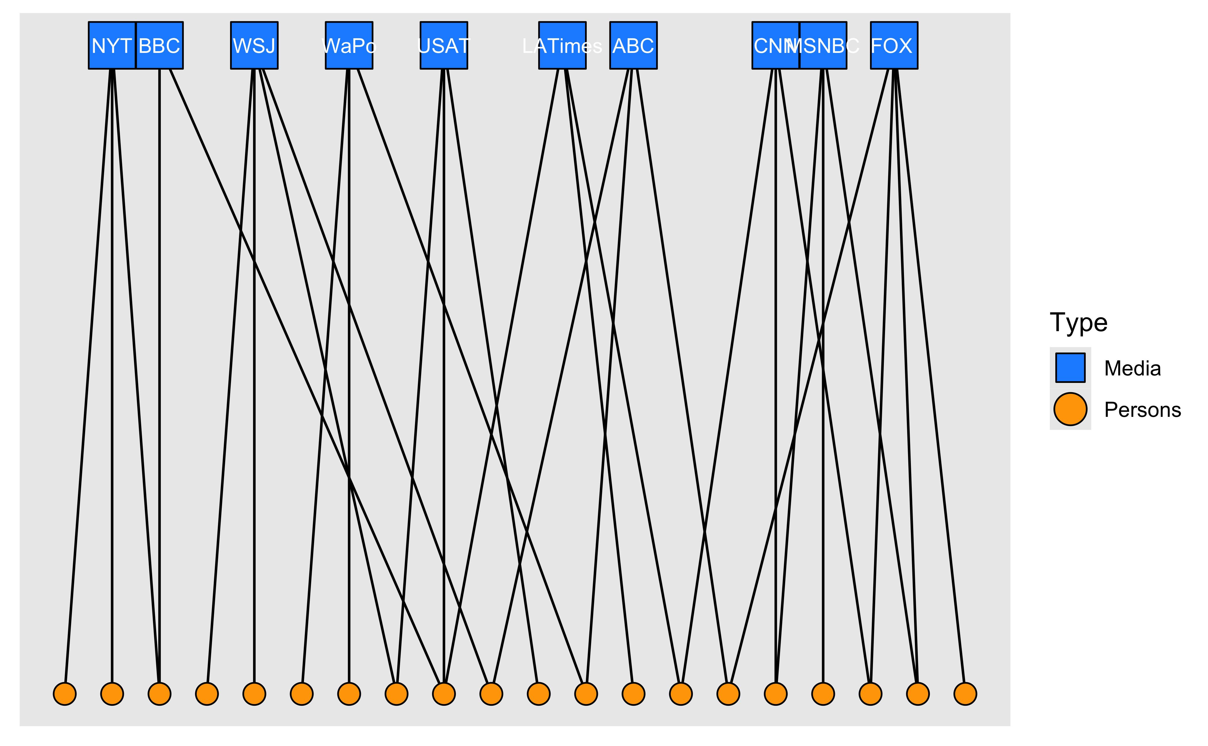

Using text as nodes:

par(mar = c(0, 0, 0, 0))
plot(net2,
  vertex.shape = "none", vertex.label = nodes2$media,
  vertex.label.color = V(net2)$color, vertex.label.font = 2,
  vertex.label.cex = .95, edge.color = "gray70", edge.width = 2
)

# Using tidygraph
as_tbl_graph(x = links2, directed = TRUE) %>%
  activate(nodes) %>%
  left_join(nodes2, by = c("name" = "id")) %>%
  ggraph(layout = "nicely") +
  geom_edge_link(
    end_cap = circle(.4, "cm"),
    start_cap = circle(0.4, "cm")
  ) +
  # geom_node>point(aes(shape = type, fill = type, size = type)) +
  geom_node_text(aes(label = media, colour = type), size = 4) +

  scale_shape_manual(
    "Type",
    values = c(22, 21),
    labels = c("Media", "Persons"),
    guide = guide_legend(override.aes = list(size = 4))
  ) +

  scale_fill_manual(
    "Type",
    values = c("dodgerblue", "orange"),
    labels = c("Media", "Persons")
  ) +

  scale_size_manual(values = c(10, 4), guide = "none")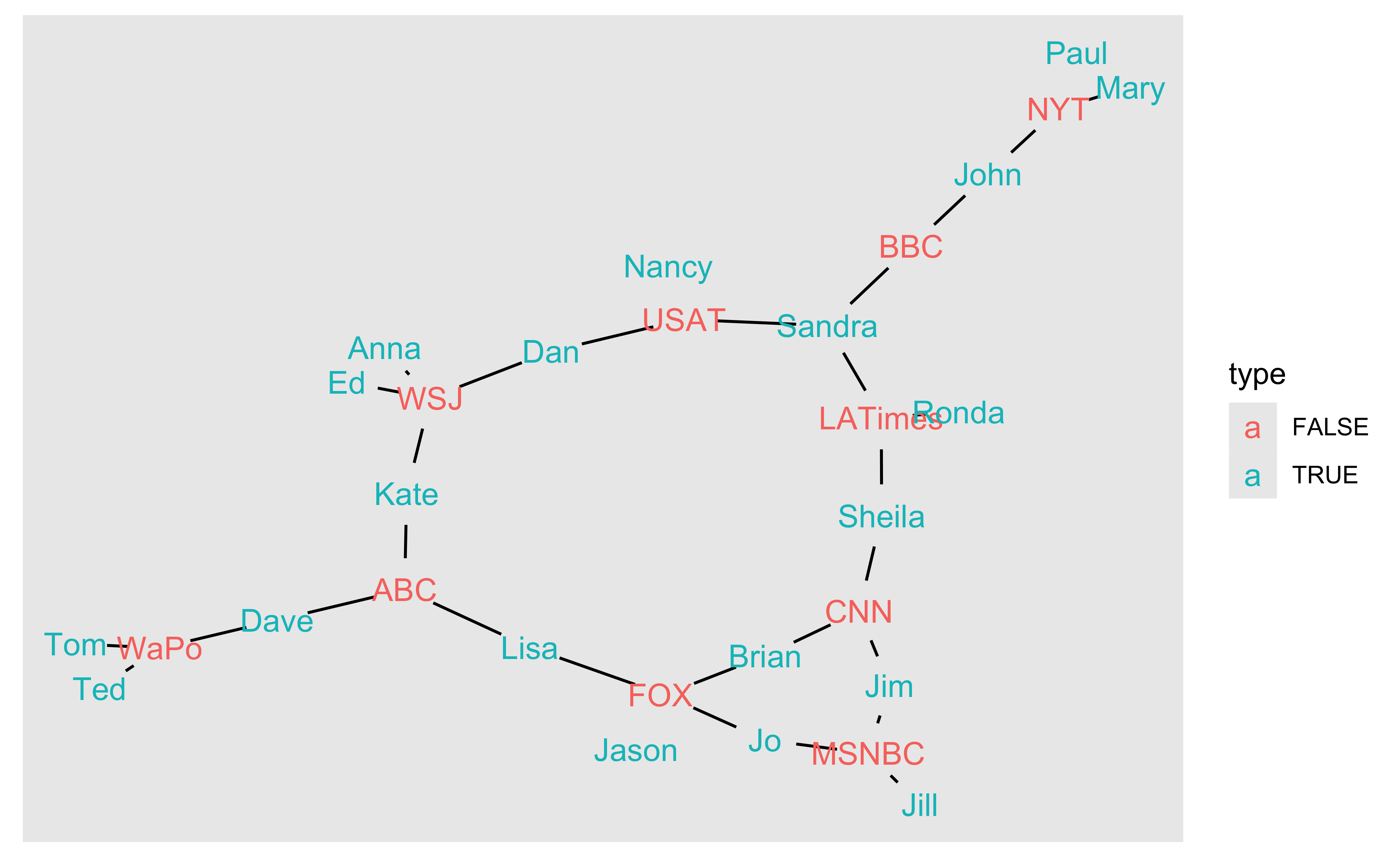

Using images as nodes You will need the ‘png’ package to do this:

# install.packages("png")
library("png")

img.1 <- readPNG("./images/news.png")
img.2 <- readPNG("./images/user.png")

V(net2)$raster <- list(img.1, img.2)[V(net2)$type + 1]

par(mar = c(3, 3, 3, 3))

plot(net2,
  vertex.shape = "raster", vertex.label = NA,
  vertex.size = 16, vertex.size2 = 16, edge.width = 2
)


# By the way, you can also add any image you want to any plot. For example, many #network graphs could be improved by a photo of a puppy carrying a basket full of kittens.
img.3 <- readPNG("./images/puppy.png")
rasterImage(img.3, xleft = -1.7, xright = 0, ybottom = -1.2, ytop = 0)

# The numbers after the image are coordinates for the plot.
# The limits of your plotting area are given in par()$usr

# Using ~~tidygraph~~ visNetwork
# See this cheatsheet:
# system.file("fontAwesome/Font_Awesome_Cheatsheet.pdf", package = "visNetwork")
library(visNetwork)

as_tbl_graph(x = links2, directed = TRUE) %>%
  activate(nodes) %>%
  left_join(nodes2, by = c("name" = "id")) %>%
  # visNetwork needs a "group" variable for grouping...
  mutate(group = as.character(type)) %>%
  visIgraph(.) %>%
  visGroups(
    groupname = "FALSE", shape = "icon",
    icon = list(code = "f26c", size = 75, color = "orange")
  ) %>%
  visGroups(
    groupname = "TRUE", shape = "icon",
    icon = list(code = "f007", size = 75)
  ) %>%
  addFontAwesome()

We can also generate and plot bipartite projections for the two-mode network : (co-memberships are easy to calculate by multiplying the network matrix by its transposed matrix, or using igraph’s bipartite.projection function)

net2.bp <- bipartite.projection(net2)

# We can calculate the projections manually as well:
as_incidence_matrix(net2) %*% t(as_incidence_matrix(net2))

    s01 s02 s03 s04 s05 s06 s07 s08 s09 s10
s01   3   0   0   0   0   0   0   0   0   1
s02   0   3   0   0   0   0   0   0   1   0
s03   0   0   4   1   0   0   0   0   1   0
s04   0   0   1   3   1   0   0   0   0   1
s05   0   0   0   1   3   1   0   0   0   1
s06   0   0   0   0   1   3   1   1   0   0
s07   0   0   0   0   0   1   3   1   0   0
s08   0   0   0   0   0   1   1   4   1   0
s09   0   1   1   0   0   0   0   1   3   0
s10   1   0   0   1   1   0   0   0   0   2

t(as_incidence_matrix(net2)) %*% as_incidence_matrix(net2)

    U01 U02 U03 U04 U05 U06 U07 U08 U09 U10 U11 U12 U13 U14 U15 U16 U17 U18 U19
U01   2   1   1   0   0   0   0   0   0   0   1   0   0   0   0   0   0   0   0
U02   1   1   1   0   0   0   0   0   0   0   0   0   0   0   0   0   0   0   0
U03   1   1   1   0   0   0   0   0   0   0   0   0   0   0   0   0   0   0   0
U04   0   0   0   1   1   0   0   0   0   0   0   0   0   0   0   0   0   0   0
U05   0   0   0   1   1   0   0   0   0   0   0   0   0   0   0   0   0   0   0
U06   0   0   0   0   0   2   1   1   1   0   0   0   0   0   0   0   0   0   1
U07   0   0   0   0   0   1   1   1   1   0   0   0   0   0   0   0   0   0   0
U08   0   0   0   0   0   1   1   1   1   0   0   0   0   0   0   0   0   0   0
U09   0   0   0   0   0   1   1   1   2   1   1   0   0   0   0   0   0   0   0
U10   0   0   0   0   0   0   0   0   1   1   1   0   0   0   0   0   0   0   0
U11   1   0   0   0   0   0   0   0   1   1   3   1   1   0   0   0   0   0   0
U12   0   0   0   0   0   0   0   0   0   0   1   1   1   0   0   0   0   0   0
U13   0   0   0   0   0   0   0   0   0   0   1   1   2   1   0   0   1   0   0
U14   0   0   0   0   0   0   0   0   0   0   0   0   1   2   1   1   1   0   0
U15   0   0   0   0   0   0   0   0   0   0   0   0   0   1   1   1   0   0   0
U16   0   0   0   0   0   0   0   0   0   0   0   0   0   1   1   2   1   1   1
U17   0   0   0   0   0   0   0   0   0   0   0   0   1   1   0   1   2   1   1
U18   0   0   0   0   0   0   0   0   0   0   0   0   0   0   0   1   1   1   1
U19   0   0   0   0   0   1   0   0   0   0   0   0   0   0   0   1   1   1   2
U20   0   0   0   1   1   1   0   0   0   0   0   0   0   0   0   0   0   0   1
    U20
U01   0
U02   0
U03   0
U04   1
U05   1
U06   1
U07   0
U08   0
U09   0
U10   0
U11   0
U12   0
U13   0
U14   0
U15   0
U16   0
U17   0
U18   0
U19   1
U20   2

par(mfrow = c(1, 2))

plot(
  net2.bp$proj1,
  vertex.label.color = "black",
  vertex.label.dist = 2,
  vertex.label = nodes2$media[!is.na(nodes2$media.type)]
)

plot(
  net2.bp$proj2,
  vertex.label.color = "black",
  vertex.label.dist = 2,
  vertex.label = nodes2$media[is.na(nodes2$media.type)]
)

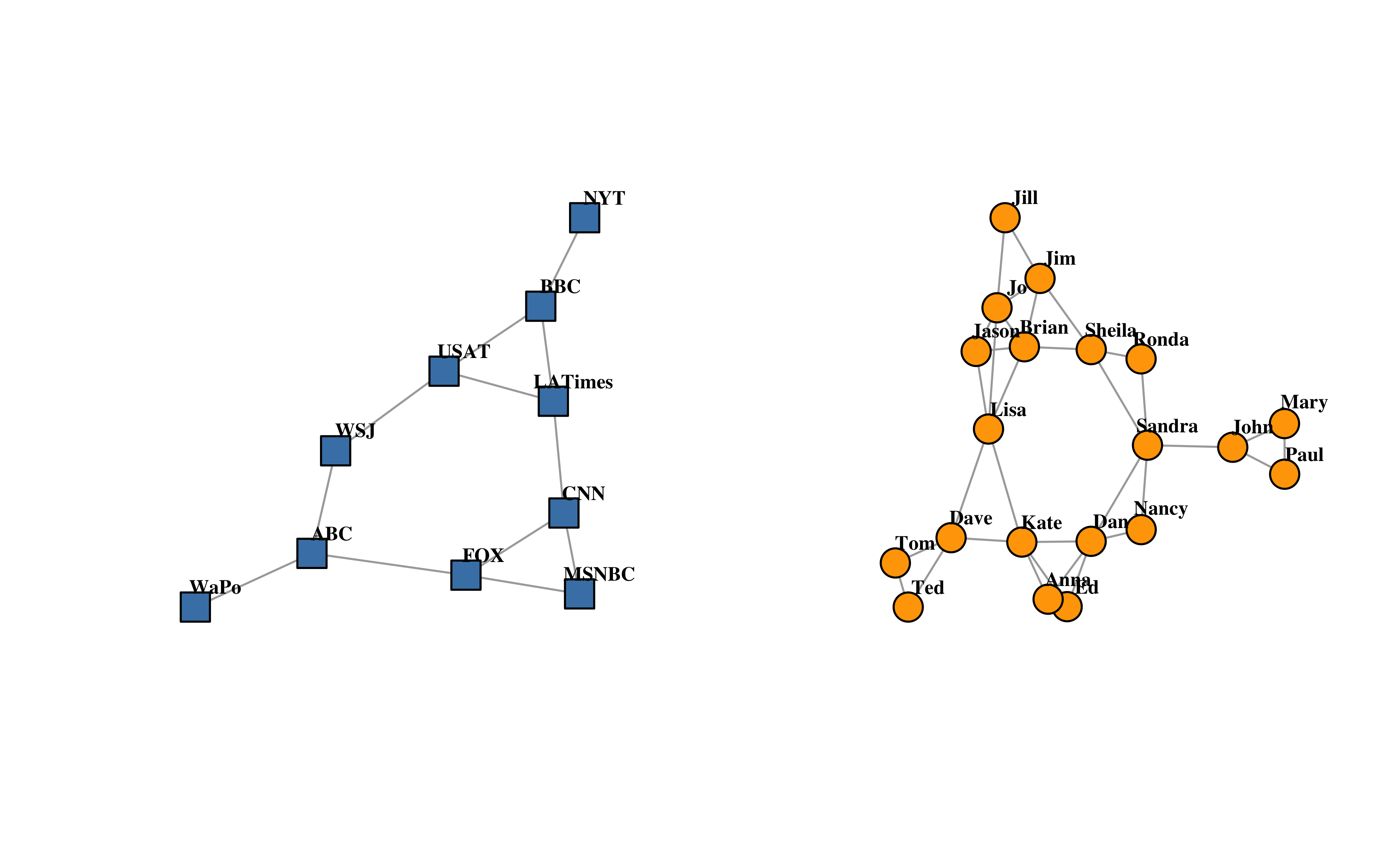
# Using tidygraph
# Calculate projections and add attributes/labels
proj1 <-
  as_incidence_matrix(net2) %*% t(as_incidence_matrix(net2)) %>%
  as_tbl_graph() %>%
  activate(nodes) %>%
  left_join(., nodes2, by = c("name" = "id"))
proj2 <-
  t(as_incidence_matrix(net2)) %*% as_incidence_matrix(net2) %>%
  as_tbl_graph() %>%
  activate(nodes) %>%
  left_join(., nodes2, by = c("name" = "id"))


p1 <- proj1 %>%
  ggraph(layout = "graphopt") +
  geom_edge_link0() +
  geom_node_point(size = 6, colour = "orange") +
  geom_node_text(aes(label = media), repel = TRUE)

p2 <- proj2 %>%
  ggraph(layout = "graphopt") +
  geom_edge_link0() +
  geom_node_point(
    aes(colour = media.type),
    size = 6,
    shape = 15,
    colour = "dodgerblue"
  ) +
  geom_node_text(aes(label = media), repel = TRUE)

p1 + p2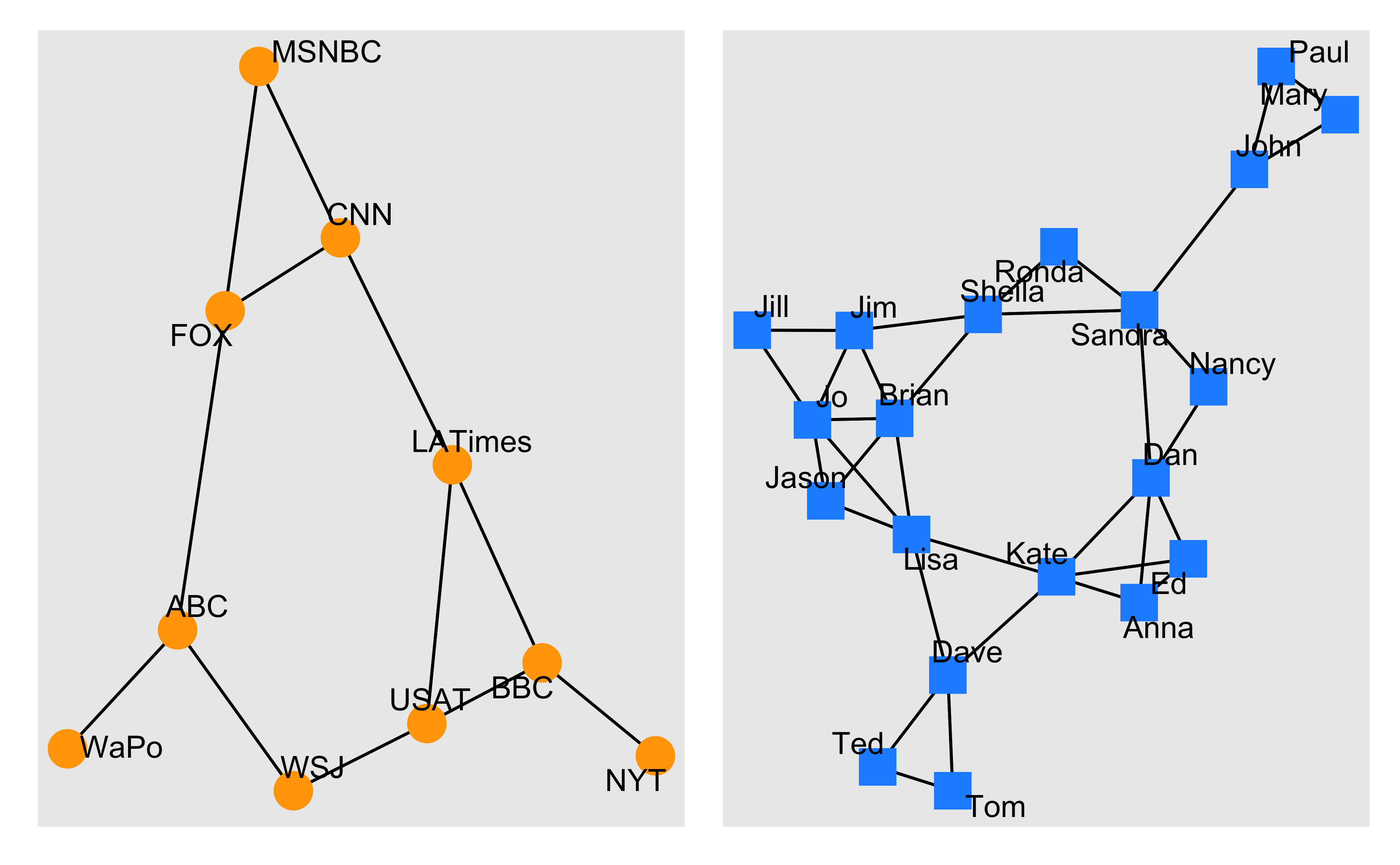

5. Plotting multiplex networks

In some cases, the networks we want to plot are multigraphs: they can have multiple edges connecting the same two nodes. A related concept, multiplex networks, contain multiple types of ties – e.g. friendship, romantic, and work relationships between individuals.

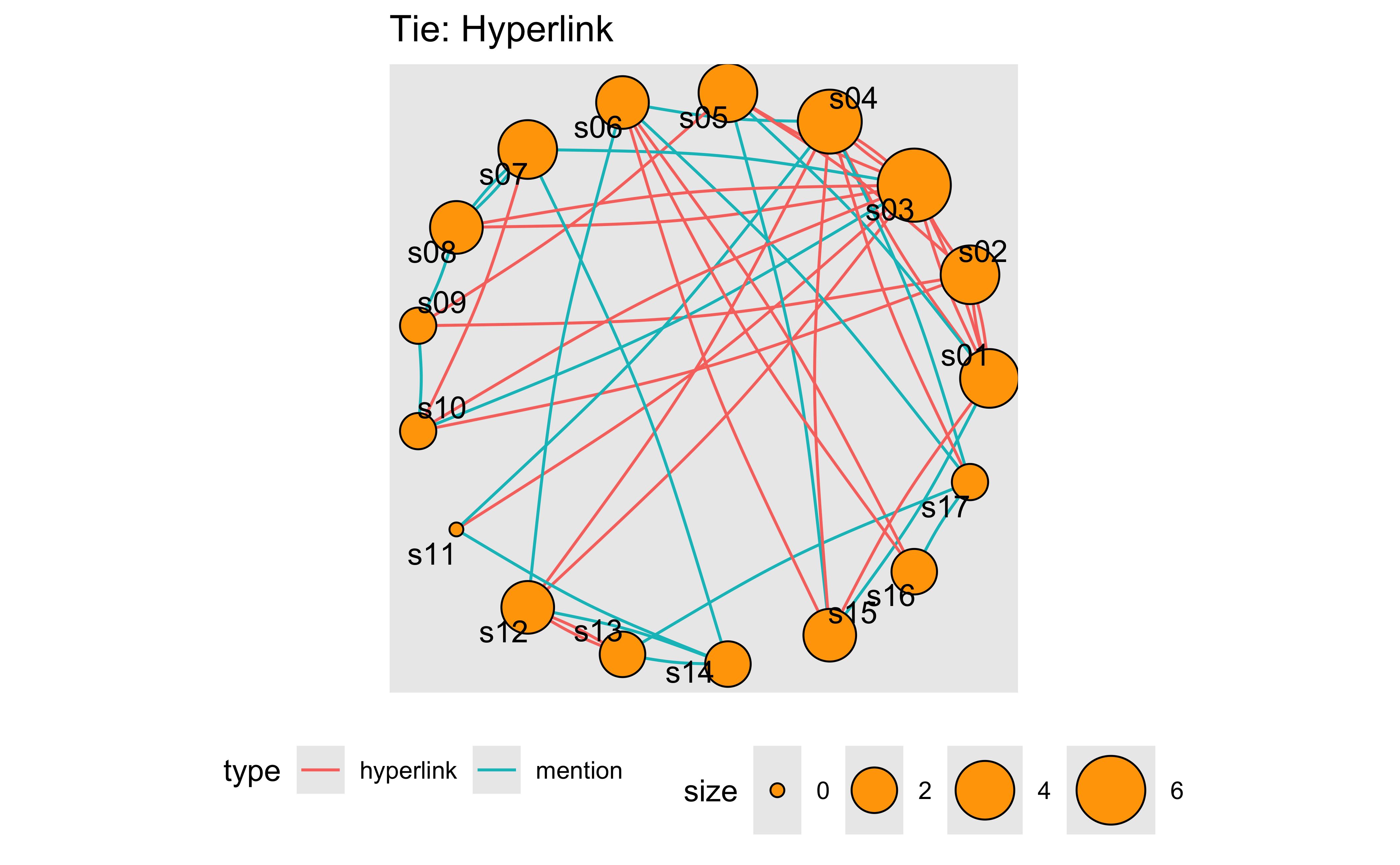
In our example network, we also have two tie types: hyperlinks and mentions. One thing we can do is plot each type of tie separately:

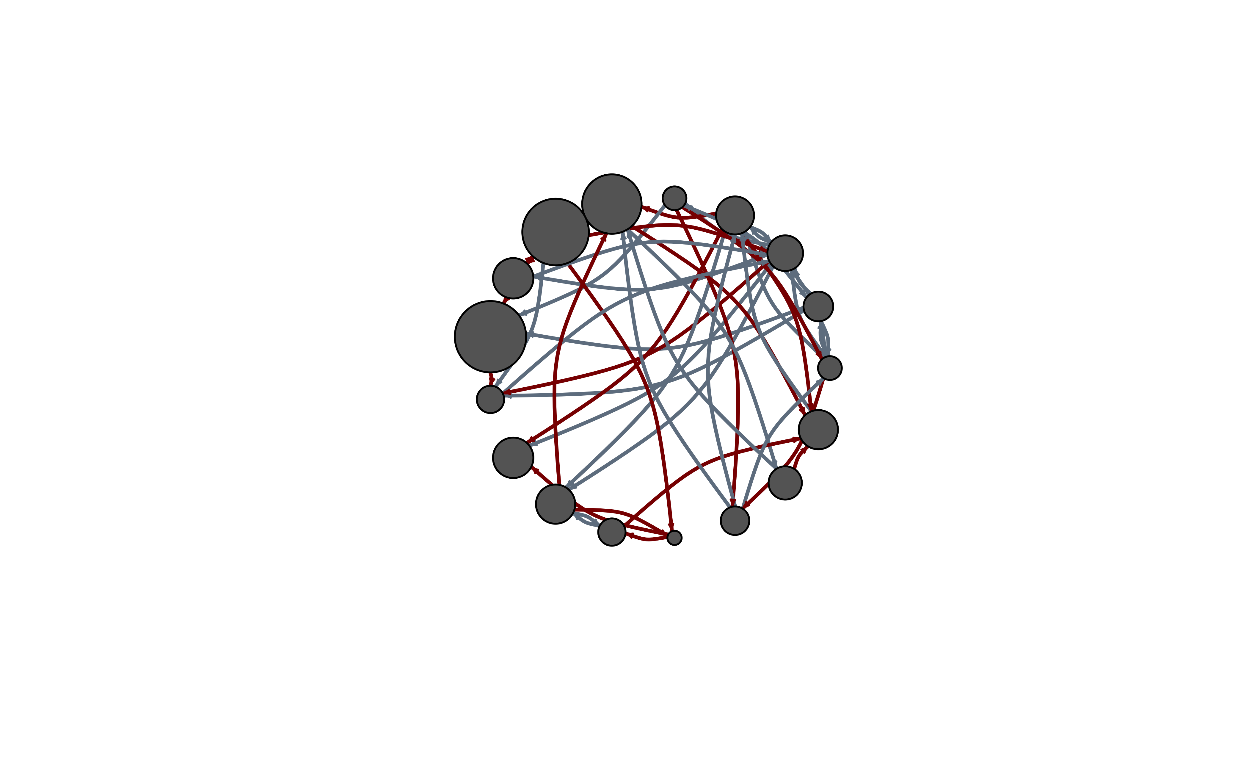
E(net)$width <- 2
plot(
  net,
  edge.color = c("dark red", "slategrey")[(E(net)$type == "hyperlink") +
    1],
  vertex.color = "gray40",
  layout = layout_in_circle,
  edge.curved = .3
)

# Another way to delete edges using the minus operator:
net.m <- net - E(net)[E(net)$type == "hyperlink"]
net.h <- net - E(net)[E(net)$type == "mention"]

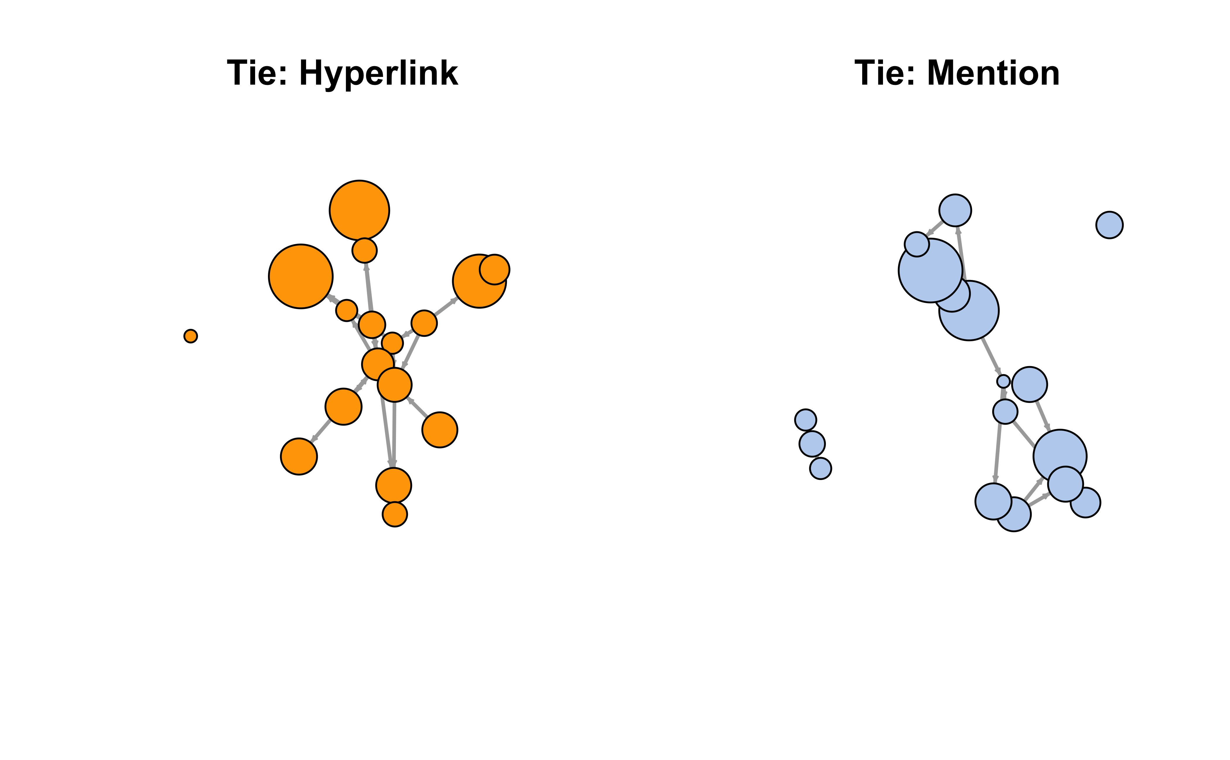
# Plot the two links separately:
par(mfrow = c(1, 2))

plot(net.h,
  vertex.color = "orange",
  layout = layout_with_fr,
  main = "Tie: Hyperlink"
)
plot(net.m,
  vertex.color = "lightsteelblue2",
  layout = layout_with_fr,
  main = "Tie: Mention"
)

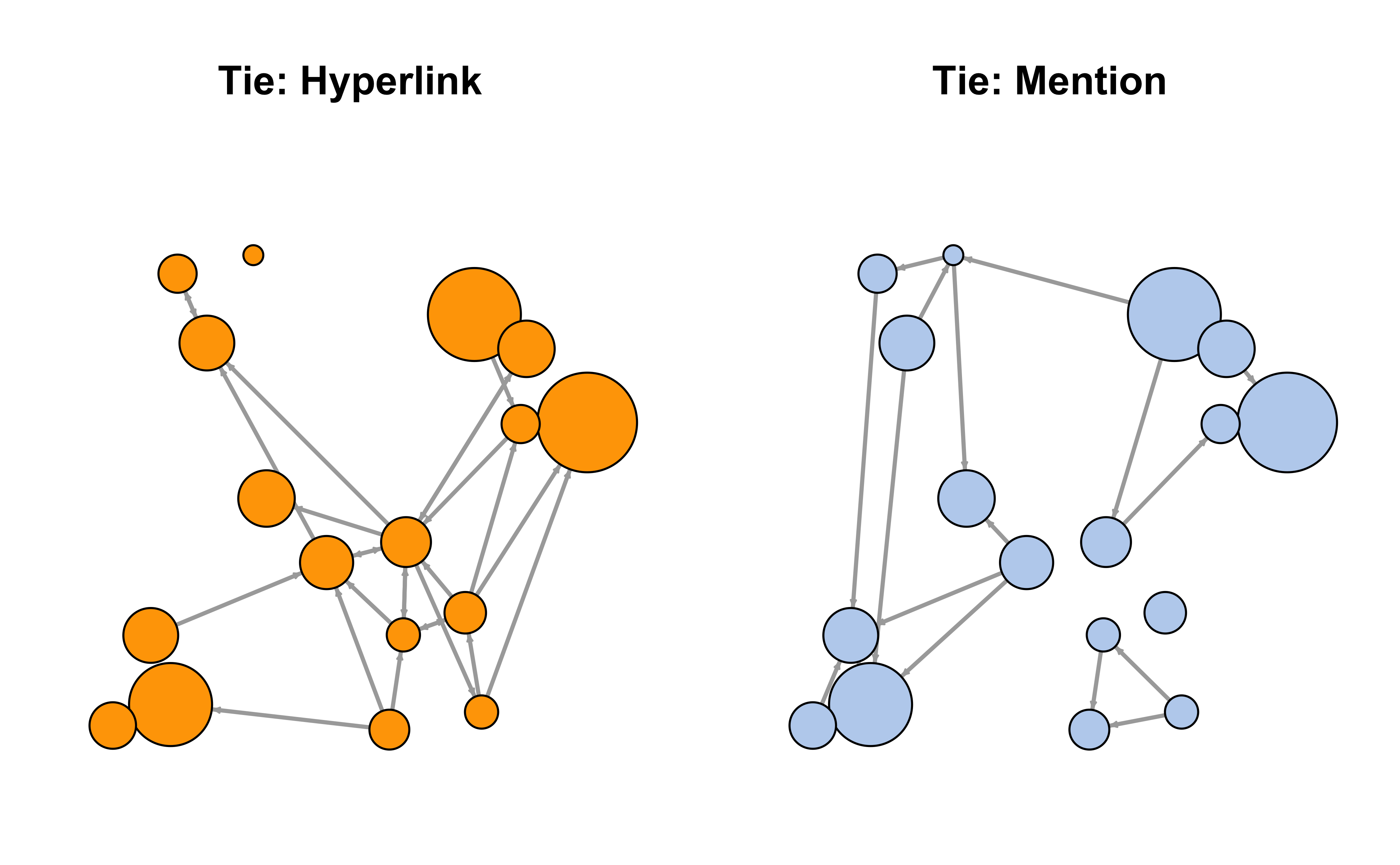
Make sure the nodes stay in the same place in both plots:

par(mfrow = c(1, 2), mar = c(1, 1, 4, 1))

l <- layout_with_fr(net)
plot(net.h,
  vertex.color = "orange",
  layout = l,
  main = "Tie: Hyperlink"
)
plot(net.m,
  vertex.color = "lightsteelblue2",
  layout = l,
  main = "Tie: Mention"
)

# Using tidygraph

layout <- layout_in_circle(net)
p1 <- tbl_graph(nodes, links, directed = TRUE) %>%
  activate(nodes) %>%
  mutate(size = centrality_degree()) %>%
  activate(edges) %>%
  filter(type == "hyperlink") %>%
  # reusing the earlier computed layout
  ggraph(layout = layout) +
  geom_edge_arc(strength = 0.05) +
  geom_node_point(aes(size = size),
    shape = 21,
    fill = "orange"
  ) +
  scale_size(range = c(2, 12)) +
  labs(title = "Tie: Hyperlink") +
  theme(
    aspect.ratio = 1, ,
    legend.position = "bottom"
  )

p2 <- tbl_graph(nodes, links, directed = TRUE) %>%
  activate(nodes) %>%
  mutate(size = centrality_degree()) %>%
  activate(edges) %>%
  filter(type == "mention") %>%
  # reusing the earlier computed layout
  ggraph(layout = layout) +
  geom_edge_arc(strength = 0.05) +
  geom_node_point(aes(size = size),
    shape = 21,
    fill = "lightsteelblue2"
  ) +
  scale_size(range = c(2, 12)) +
  labs(title = "Tie: Mention") +
  theme(aspect.ratio = 1, legend.position = "bottom")

wrap_plots(p1, p2, guides = "collect") &
  # note this "pipe" for patchwork!
  theme(legend.position = "none")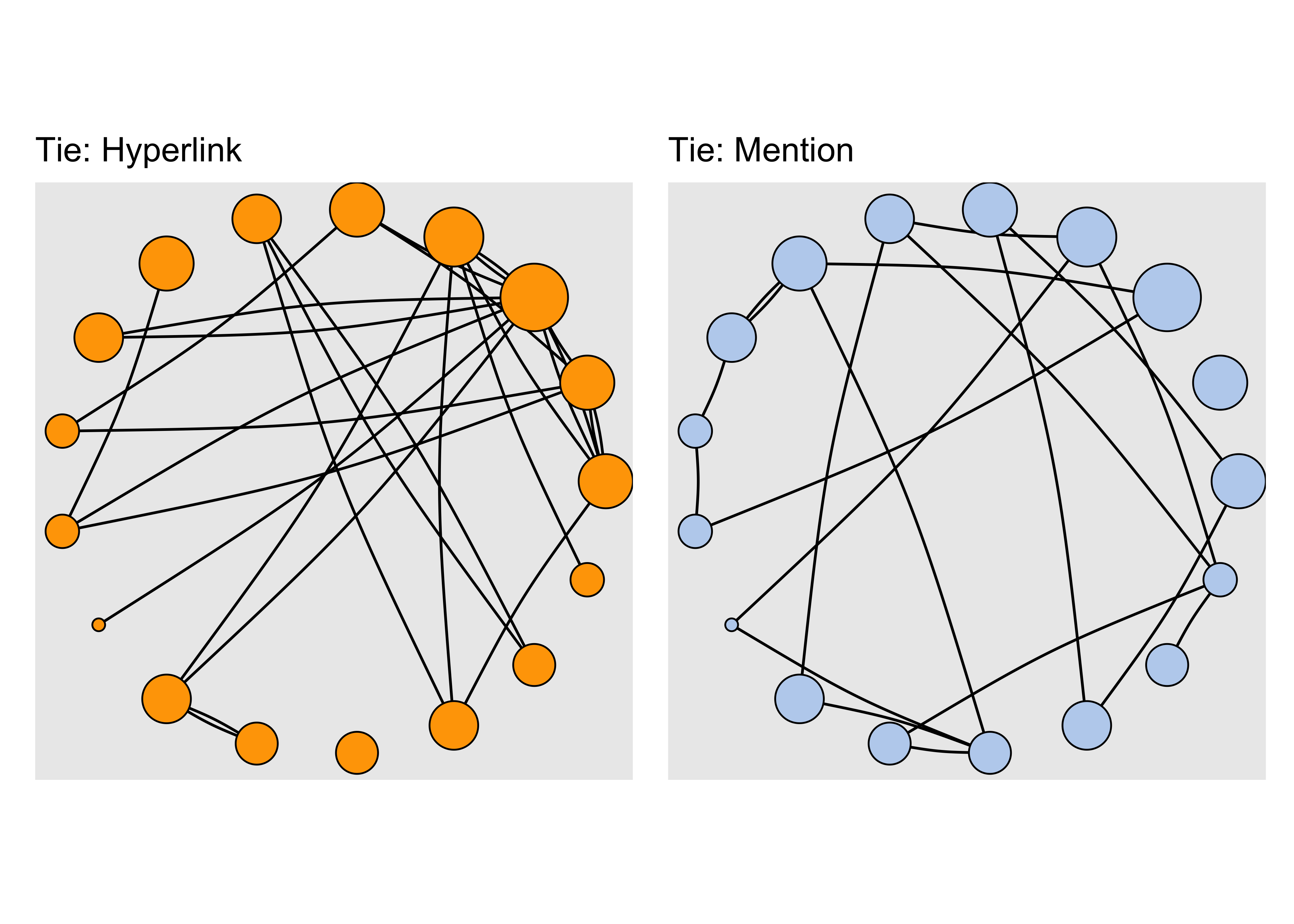

In our example network, we don’t have node dyads connected by multiple types of connections (we never have both a ‘hyperlink’ and a ‘mention’ tie between the same two news outlets) – however that could happen.

Note: See the edges between s03 and s10…these are in opposite directions. So no dyads.

layout <- layout_in_circle(net)
tbl_graph(nodes, links, directed = TRUE) %>%
  activate(nodes) %>%
  mutate(size = centrality_degree()) %>%
  # reusing the earlier computed layout
  ggraph(layout = layout) +
  geom_edge_arc(strength = 0.05, aes(colour = type)) +
  geom_node_point(aes(size = size),
    shape = 21,
    fill = "orange"
  ) +
  geom_node_text(aes(label = id), repel = TRUE) +
  scale_size(range = c(2, 12)) +
  labs(title = "Tie: Hyperlink") +
  theme(
    aspect.ratio = 1, ,
    legend.position = "bottom"
  )

One challenge in visualizing multiplex networks is that multiple edges between the same two nodes may get plotted on top of each other in a way that makes them impossible to distinguish. For example, let us generate a simple multiplex network with two nodes and three ties between them:

multigtr <- graph(edges = c(1, 2, 1, 2, 1, 2), n = 2)

l <- layout_with_kk(multigtr)

# Let's just plot the graph:
plot(
  multigtr,
  vertex.color = "lightsteelblue",
  vertex.frame.color = "white",
  vertex.size = 40,
  vertex.shape = "circle",
  vertex.label = NA,
  edge.color = c("gold", "tomato", "yellowgreen"),
  edge.width = 10,
  edge.arrow.size = 5,
  edge.curved = 0.1,
  layout = l
)

# Using tidygraph
multigtr %>%
  as_tbl_graph() %>%
  activate(edges) %>%
  mutate(edge_col = c("gold", "tomato", "yellowgreen")) %>%
  ggraph(., layout = l) +
  geom_edge_arc(strength = 0.1, aes(colour = edge_col)) +
  geom_node_point(size = 4, colour = "lightsteelblue") +
  theme(legend.position = "none")

Because all edges in the graph have the same curvature, they are drawn over each other so that we only see the last one. What we can do is assign each edge a different curvature. One useful function in ‘igraph’ called curve_multiple() can help us here. For a graph G, curve.multiple(G) will generate a curvature for each edge that maximizes visibility.

plot(
  multigtr,
  vertex.color = "lightsteelblue",
  vertex.frame.color = "white",
  vertex.size = 40,
  vertex.shape = "circle",
  vertex.label = NA,
  edge.color = c("gold", "tomato", "yellowgreen"),
  edge.width = 10,
  edge.arrow.size = 5,
  edge.curved = curve_multiple(multigtr),
  layout = l
)

multigtr %>%
  as_tbl_graph() %>%
  activate(edges) %>%
  mutate(edge_col = c("gold", "tomato", "yellowgreen")) %>%
  ggraph(., layout = l) +
  geom_edge_fan(strength = 0.1, aes(colour = edge_col), width = 2) +
  geom_node_point(size = 4, colour = "lightsteelblue") +
  theme(legend.position = "none")

And that is the end of this reoworked tutorial! Hope you enjoyed it and found it useful!!

Introduction

CONTENTS

——-~~ DATASET 1: edgelist ~~——-

Converting the data to an igraph object:

——-~~ DATASET 2: matrix ——–

3. Network plots in ‘igraph’

——~~ Plot parameters in igraph ——–

——-~~ Network Layouts in ‘igraph’ ——–

——-~~ Highlighting aspects of the network ——–

Community Detection

——-~~ Highlighting specific nodes or links ——–

Path Highlighting

Highlight Neighbours

——-~~ Interactive plotting with ‘tkplot’ ——–

——-~~ Other ways to represent a network ——–

4. Plotting two-mode networks

5. Plotting multiplex networks

——- DATASET 1: edgelist ——-