Tutorial: Multiple Linear Regression with Backward Selection

Linear Regression

Quantitative Predictor

Quantitative Response

Sum of Squares

Residuals

Author

Arvind V.

Published

May 3, 2023

Modified

May 21, 2024

Abstract

Using Multiple Regression to predict Quantitative Target Variables

Setting up R Packages

options(scipen = 1, digits = 3) #set to three decimal 
knitr::opts_chunk$set(echo = TRUE,warning = FALSE,message = FALSE)
library(tidyverse)
library(ggformula)
library(mosaic)
library(infer)

# Let us set a plot theme for Data visualisation

# my_theme <- function(){  # Creating a function
#   theme_classic() +  # Using pre-defined theme as base
#   theme(axis.text.x = element_text(size = 12, face = "bold"),  # Customizing axes text      
#         axis.text.y = element_text(size = 12, face = "bold"),
#         axis.title = element_text(size = 14, face = "bold"),  # Customizing axis title
#         panel.grid = element_blank(),  # Taking off the default grid
#         plot.margin = unit(c(0.5, 0.5, 0.5, 0.5), units = , "cm"),
#         legend.text = element_text(size = 12, face = "italic"),  # Customizing legend text
#         legend.title = element_text(size = 12, face = "bold"),  # Customizing legend title
#         legend.position = "right",  # Customizing legend position
#         plot.caption = element_text(size = 12))  # Customizing plot caption
# }   

my_theme <- function(){  # Creating a function
  theme_classic() +  # Using pre-defined theme as base
  theme(plot.title = element_text(face = "bold", size = 14),
        axis.text.x = element_text(size = 10, face = "bold"),  
        # Customizing axes text      
        axis.text.y = element_text(size = 10, face = "bold"),
        axis.title = element_text(size = 12, face = "bold"),  
        # Customizing axis title
        panel.grid = element_blank(),  # Taking off the default grid
        plot.margin = unit(c(0.5, 0.5, 0.5, 0.5), units = , "cm"),
        legend.text = element_text(size = 8, face = "italic"),  
        # Customizing legend text
        legend.title = element_text(size = 10, face = "bold"),  
        # Customizing legend title
        legend.position = "right",  # Customizing legend position
        plot.caption = element_text(size = 8))  # Customizing plot caption
}

In this tutorial, we will use the Boston housing dataset. Our research question is:

Research Question

How do we predict the price of a house in Boston, based on other parameters Quantitative parameters such as area, location, rooms, and crime-rate in the neighbourhood?

And how do we choose the “best” model, based on a tradeoff between Model Complexity and Model Accuracy?

Workflow: Read the Data

data("BostonHousing2", package = "mlbench")
housing <- BostonHousing2
inspect(housing)


categorical variables:  
  name  class levels   n missing                                  distribution
1 town factor     92 506       0 Cambridge (5.9%) ...                         
2 chas factor      2 506       0 0 (93.1%), 1 (6.9%)                          

quantitative variables:  
      name   class       min       Q1   median       Q3      max     mean
1    tract integer   1.00000 1303.250 3393.500 3739.750 5082.000 2700.356
2      lon numeric -71.28950  -71.093  -71.053  -71.020  -70.810  -71.056
3      lat numeric  42.03000   42.181   42.218   42.252   42.381   42.216
4     medv numeric   5.00000   17.025   21.200   25.000   50.000   22.533
5    cmedv numeric   5.00000   17.025   21.200   25.000   50.000   22.529
6     crim numeric   0.00632    0.082    0.257    3.677   88.976    3.614
7       zn numeric   0.00000    0.000    0.000   12.500  100.000   11.364
8    indus numeric   0.46000    5.190    9.690   18.100   27.740   11.137
9      nox numeric   0.38500    0.449    0.538    0.624    0.871    0.555
10      rm numeric   3.56100    5.886    6.208    6.623    8.780    6.285
11     age numeric   2.90000   45.025   77.500   94.075  100.000   68.575
12     dis numeric   1.12960    2.100    3.207    5.188   12.127    3.795
13     rad integer   1.00000    4.000    5.000   24.000   24.000    9.549
14     tax integer 187.00000  279.000  330.000  666.000  711.000  408.237
15 ptratio numeric  12.60000   17.400   19.050   20.200   22.000   18.456
16       b numeric   0.32000  375.377  391.440  396.225  396.900  356.674
17   lstat numeric   1.73000    6.950   11.360   16.955   37.970   12.653
          sd   n missing
1  1380.0368 506       0
2     0.0754 506       0
3     0.0618 506       0
4     9.1971 506       0
5     9.1822 506       0
6     8.6015 506       0
7    23.3225 506       0
8     6.8604 506       0
9     0.1159 506       0
10    0.7026 506       0
11   28.1489 506       0
12    2.1057 506       0
13    8.7073 506       0
14  168.5371 506       0
15    2.1649 506       0
16   91.2949 506       0
17    7.1411 506       0

The original data are 506 observations on 14 variables, medv being the target variable:

crim	per capita crime rate by town
zn	proportion of residential land zoned for lots over 25,000 sq.ft
indus	proportion of non-retail business acres per town
chas	Charles River dummy variable (= 1 if tract bounds river; 0 otherwise)
nox	nitric oxides concentration (parts per 10 million)
rm	average number of rooms per dwelling
age	proportion of owner-occupied units built prior to 1940
dis	weighted distances to five Boston employment centres
rad	index of accessibility to radial highways
tax	full-value property-tax rate per USD 10,000
ptratio	pupil-teacher ratio by town
b	$1000 (B - 0.63)^{2}$ where B is the proportion of Blacks by town
lstat	percentage of lower status of the population
medv	median value of owner-occupied homes in USD 1000’s

The corrected data set has the following additional columns:

cmedv	corrected median value of owner-occupied homes in USD 1000’s
town	name of town
tract	census tract
lon	longitude of census tract
lat	latitude of census tract

Our response variable is cmedv, the corrected median value of owner-occupied homes in USD 1000’s. Their are many Quantitative feature variables that we can use to predict cmedv. And there are two Qualitative features, chas and tax.

Workflow: Correlations

We can use purrr to evaluate all pair-wise correlations in one shot:

all_corrs <- housing %>% 
  select(where(is.numeric)) %>% 
  
  # leave off cmedv/medv to get all the remaining ones
  select(- cmedv, -medv) %>%  
  
  # perform a cor.test for all variables against cmedv
  purrr::map(.x = .,
             .f = \(x) cor.test(x, housing$cmedv)) %>%
  
  # tidy up the cor.test outputs into a tidy data frame
  map_dfr(broom::tidy, .id = "predictor") 

all_corrs

ABCDEFGHIJ0123456789

predictor <chr>	estimate <dbl>	statistic <dbl>	p.value <dbl>	parameter <int>	conf.low <dbl>	conf.high <dbl>	method <chr>
tract	0.42825	10.639	5.51e-24	504	0.3543	0.4969	Pearson's product-moment correlation
lon	-0.32295	-7.661	9.55e-14	504	-0.3989	-0.2426	Pearson's product-moment correlation
lat	0.00683	0.153	8.78e-01	504	-0.0804	0.0939	Pearson's product-moment correlation
crim	-0.38958	-9.496	8.71e-20	504	-0.4611	-0.3130	Pearson's product-moment correlation
zn	0.36039	8.673	5.79e-17	504	0.2821	0.4339	Pearson's product-moment correlation
indus	-0.48475	-12.442	3.52e-31	504	-0.5487	-0.4151	Pearson's product-moment correlation
nox	-0.42930	-10.671	4.17e-24	504	-0.4978	-0.3554	Pearson's product-moment correlation
rm	0.69630	21.779	1.31e-74	504	0.6485	0.7386	Pearson's product-moment correlation
age	-0.37800	-9.166	1.24e-18	504	-0.4503	-0.3007	Pearson's product-moment correlation
dis	0.24931	5.780	1.31e-08	504	0.1657	0.3293	Pearson's product-moment correlation

all_corrs %>%
  gf_hline(yintercept = 0,
           color = "grey",
           linewidth = 2) %>%
  gf_errorbar(
    conf.high + conf.low ~ reorder(predictor, estimate),
    colour = ~ estimate,
    width = 0.5,
    linewidth = ~ -log10(p.value),
    caption = "Significance = -log10(p.value)"
  ) %>%
  gf_point(estimate ~ reorder(predictor, estimate)) %>%
  gf_labs(x = "Predictors", y = "Correlation with Median House Price") %>%
  gf_theme(my_theme()) %>%
  gf_theme(theme(axis.text.x = element_text(angle = 45, hjust = 1))) %>%
  gf_refine(
    scale_colour_distiller("Correlation", type = "div", palette = "RdBu"),
    scale_linewidth_continuous("Significance", range = c(0.25, 3)),
    guides(linewidth = guide_legend(reverse = TRUE)))

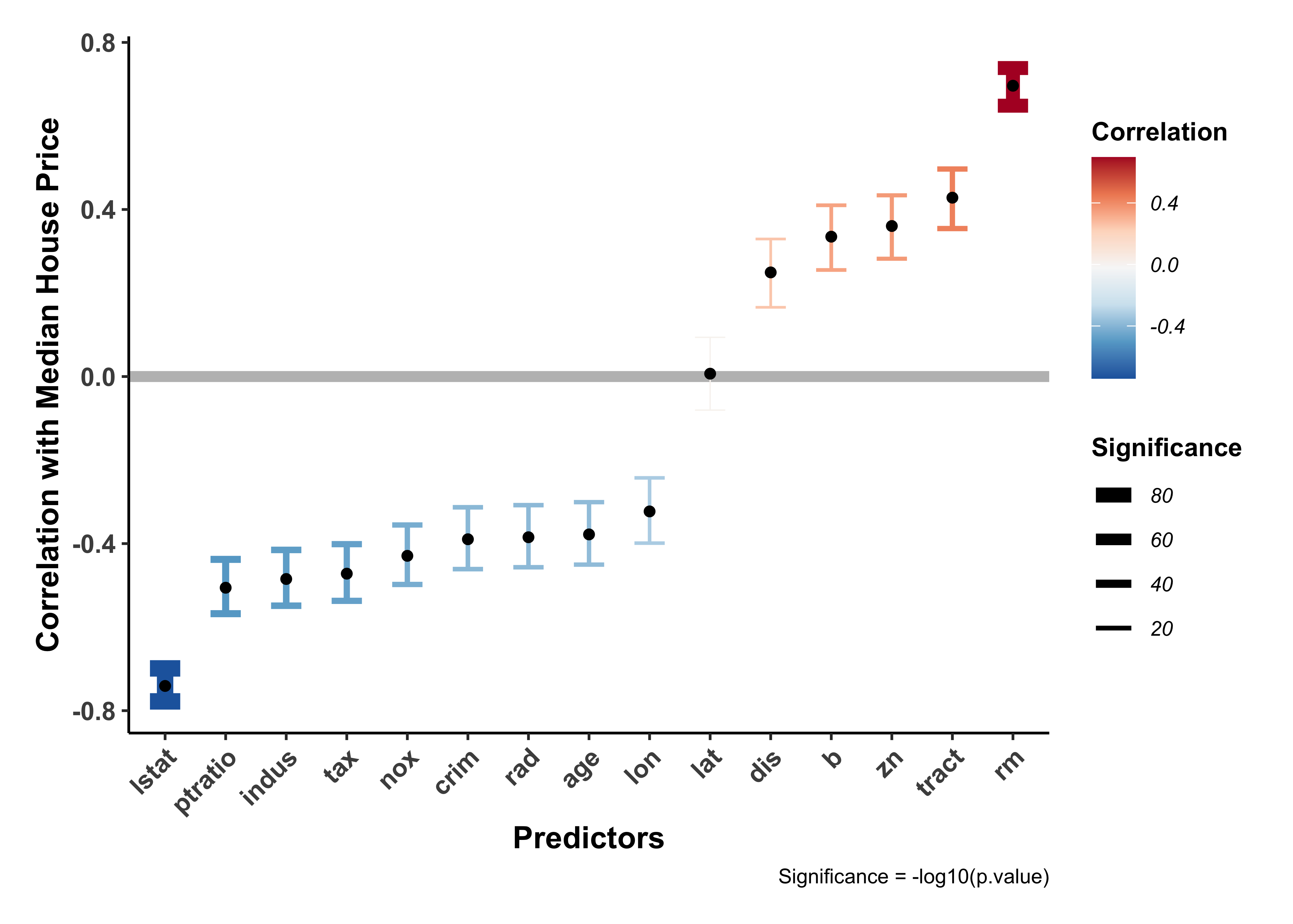
The variables rm, lstat seem to have high correlations with cmedv which are also statistically significant.

Workflow: Maximal Multiple Regression Model

We will create a regression model for cmedv using all the other numerical predictor features in the dataset.

housing_numeric <- housing %>% select(where(is.numeric), 
                                      
                    # remove medv
                    # an older version of cmedv
                                      -c(medv))
names(housing_numeric) # 16 variables, one target, 15 predictors

 [1] "tract"   "lon"     "lat"     "cmedv"   "crim"    "zn"      "indus"  
 [8] "nox"     "rm"      "age"     "dis"     "rad"     "tax"     "ptratio"
[15] "b"       "lstat"

housing_maximal <- lm(cmedv ~ ., data = housing_numeric)
summary(housing_maximal)


Call:
lm(formula = cmedv ~ ., data = housing_numeric)

Residuals:
    Min      1Q  Median      3Q     Max 
-13.934  -2.752  -0.619   1.711  26.120 

Coefficients:
             Estimate Std. Error t value Pr(>|t|)    
(Intercept) -3.45e+02   3.23e+02   -1.07  0.28734    
tract       -7.52e-04   4.46e-04   -1.69  0.09231 .  
lon         -6.79e+00   3.44e+00   -1.98  0.04870 *  
lat         -2.35e+00   5.36e+00   -0.44  0.66074    
crim        -1.09e-01   3.28e-02   -3.32  0.00097 ***
zn           4.40e-02   1.39e-02    3.17  0.00164 ** 
indus        2.75e-02   6.20e-02    0.44  0.65692    
nox         -1.55e+01   4.03e+00   -3.85  0.00014 ***
rm           3.81e+00   4.20e-01    9.07  < 2e-16 ***
age          5.82e-03   1.34e-02    0.43  0.66416    
dis         -1.38e+00   2.10e-01   -6.59  1.1e-10 ***
rad          2.36e-01   8.47e-02    2.78  0.00558 ** 
tax         -1.48e-02   3.74e-03   -3.96  8.5e-05 ***
ptratio     -9.49e-01   1.41e-01   -6.73  4.7e-11 ***
b            9.55e-03   2.67e-03    3.57  0.00039 ***
lstat       -5.46e-01   5.06e-02  -10.80  < 2e-16 ***
---
Signif. codes:  0 '***' 0.001 '**' 0.01 '*' 0.05 '.' 0.1 ' ' 1

Residual standard error: 4.73 on 490 degrees of freedom
Multiple R-squared:  0.743, Adjusted R-squared:  0.735 
F-statistic: 94.3 on 15 and 490 DF,  p-value: <2e-16

The maximal model has an R.squared of $0.7426$ which is much better than that we obtained for a simple model based on rm alone. How much can we simplify this maximal model, without losing out on R.squared?

Workflow: Model Reduction

We now proceed naively by removing one predictor after another. We will resort to what may amount to p-hacking by sorting the predictors based on their p-value¹ in the maximal model and removing them in decreasing order of their p-value.

We will also use some powerful features from the purrr package (also part of the tidyverse), to create all these models all at once. Then we will be able to plot their R.squared values together and decide where we wish to trade off Explainability vs Complexity for our model.

# No of Quant predictor variables in the dataset
n_vars <- housing %>%
  select(where(is.numeric), -c(cmedv, medv)) %>%
  length()

# Maximal Model, now tidied
housing_maximal_tidy <- 
  housing_maximal %>% 
  broom::tidy() %>% 
  
# Obviously remove "Intercept" ;-D
  filter(term != "(Intercept)") %>% 
  
# And horrors! Sort variables by p.value
  arrange(p.value)

housing_maximal_tidy

ABCDEFGHIJ0123456789

term <chr>	estimate <dbl>	std.error <dbl>	statistic <dbl>	p.value <dbl>
lstat	-0.546440	0.050619	-10.795	1.62e-24
rm	3.809475	0.419779	9.075	2.77e-18
ptratio	-0.948941	0.140991	-6.730	4.74e-11
dis	-1.384370	0.210041	-6.591	1.13e-10
tax	-0.014807	0.003737	-3.962	8.54e-05
nox	-15.506379	4.032786	-3.845	1.36e-04
b	0.009548	0.002675	3.569	3.94e-04
crim	-0.108861	0.032789	-3.320	9.67e-04
zn	0.043968	0.013883	3.167	1.64e-03
rad	0.235674	0.084665	2.784	5.58e-03

The last 5 variables are clearly statistically insignificant.

And now we unleash the purrr package to create all the simplified models at once. We will construct a dataset containing three columns:

A list of all quantitative predictor variables
A sequence of numbers from 1 to N(predictor)
A “list” column containing the housing data frame itself

We will use the iteration capability of purrr to sequentially drop one variable at a time from the maximal(15 predictor) model, build a new reduced model each time, and compute the r.squared:

housing_model_set <- tibble(all_vars = 
                            list(housing_maximal_tidy$term), # p-hacked order!!
                            keep_vars = seq(1, n_vars),
                            data = list(housing_numeric))
housing_model_set
# Unleash purrr in a series of mutates
housing_model_set <- housing_model_set %>%
  
# list of predictor variables for each model
  mutate(mod_vars =
           pmap(
             .l = list(all_vars, keep_vars, data),
             .f = \(all_vars, keep_vars, data) all_vars[1:keep_vars]
           )) %>%
  
# build formulae with these for linear regression
  mutate(formula = 
           map(.x = mod_vars,
               .f = \(mod_vars) as.formula(paste(
                         "cmedv ~", paste(mod_vars, collapse = "+")
                       )))) %>%
  
# use the formulae to build multiple linear models
  mutate(models =
           pmap(
             .l = list(data, formula),
             .f = \(data, formula) lm(formula, data = data)
           ))
# Check everything after the operation
housing_model_set
# Tidy up the models using broom to expose their metrics
housing_models_tidy <- housing_model_set %>% 
  mutate(tidy_models =
           map(
             .x = models,
             .f = \(x) broom::glance(x,
                                     conf.int = TRUE,
                                     conf.lvel = 0.95)
           )) %>% 

  # Remove unwanted columns, keep model and predictor count
  select(keep_vars, tidy_models) %>%
  unnest(tidy_models)

housing_models_tidy %>%
  gf_line(
    r.squared ~ keep_vars,
    ylab = "R.Squared",
    xlab = "No. params in the Linear Model",
    title = "Model Explainability vs Complexity",
    subtitle = "Model r.squared vs No. of Predictors",
    data = .
  ) %>%
  
  # Plot r.squared vs predictor count
  gf_point(r.squared ~ keep_vars,
           size = 3.5, color = "grey") %>%
  
  # Show off the selected best model
  gf_point(
    r.squared ~ keep_vars,
    size = 3.5,
    color = "red",
    data = housing_models_tidy %>% filter(keep_vars == 4)
  ) %>%
  
  gf_hline(yintercept = 0.7, linetype = "dashed") %>%
  gf_theme(my_theme())

ABCDEFGHIJ0123456789

all_vars <list>	keep_vars <int>	data <list>
<chr [15]>	1	<df[,16] [506 × 16]>
<chr [15]>	2	<df[,16] [506 × 16]>
<chr [15]>	3	<df[,16] [506 × 16]>
<chr [15]>	4	<df[,16] [506 × 16]>
<chr [15]>	5	<df[,16] [506 × 16]>
<chr [15]>	6	<df[,16] [506 × 16]>
<chr [15]>	7	<df[,16] [506 × 16]>
<chr [15]>	8	<df[,16] [506 × 16]>
<chr [15]>	9	<df[,16] [506 × 16]>
<chr [15]>	10	<df[,16] [506 × 16]>

ABCDEFGHIJ0123456789

all_vars <list>	keep_vars <int>	data <list>	mod_vars <list>
<chr [15]>	1	<df[,16] [506 × 16]>	<chr [1]>
<chr [15]>	2	<df[,16] [506 × 16]>	<chr [2]>
<chr [15]>	3	<df[,16] [506 × 16]>	<chr [3]>
<chr [15]>	4	<df[,16] [506 × 16]>	<chr [4]>
<chr [15]>	5	<df[,16] [506 × 16]>	<chr [5]>
<chr [15]>	6	<df[,16] [506 × 16]>	<chr [6]>
<chr [15]>	7	<df[,16] [506 × 16]>	<chr [7]>
<chr [15]>	8	<df[,16] [506 × 16]>	<chr [8]>
<chr [15]>	9	<df[,16] [506 × 16]>	<chr [9]>
<chr [15]>	10	<df[,16] [506 × 16]>	<chr [10]>

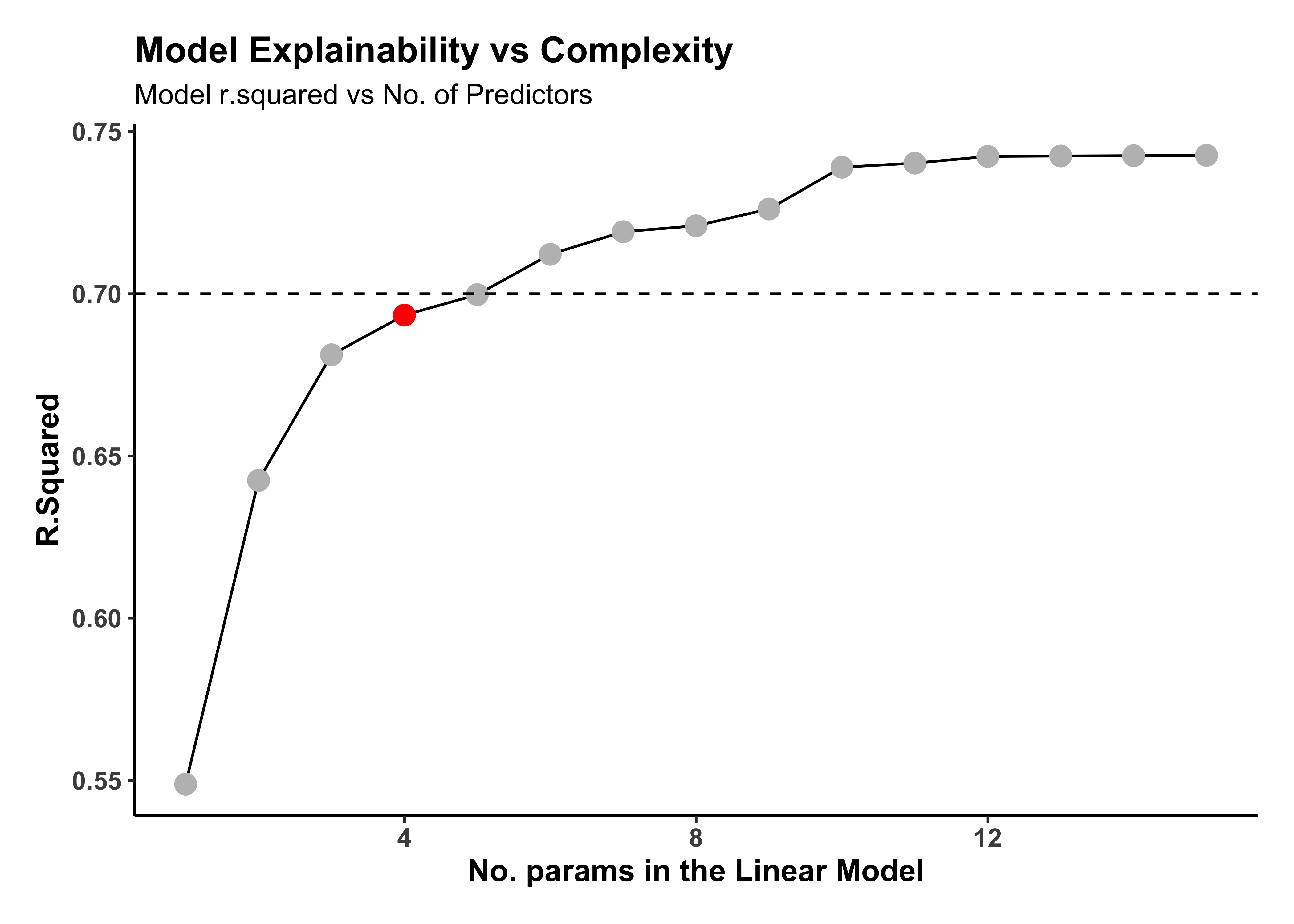
At the loss of some 5% in the r.squared, we can drop our model complexity from 15 predictors to say 4! Our final model will then be:

housing_model_final <- 
  housing_model_set %>% 
  
  # filter for best model, with 4 variables
  filter(keep_vars == 4) %>% 
  
  # tidy up the model
  mutate(tidy_models =
           map(
             .x = models,
             .f = \(x) broom::tidy(x,
                                     conf.int = TRUE,
                                     conf.lvel = 0.95)
           )) %>% 
  
  # Remove unwanted columns, keep model and predictor count
  select(keep_vars, models, tidy_models) %>%
  unnest(tidy_models)

housing_model_final

ABCDEFGHIJ0123456789

keep_vars <int>	models <list>	term <chr>	estimate <dbl>	std.error <dbl>	statistic <dbl>	p.value <dbl>	conf.low <dbl>	conf.high <dbl>
4	<S3: lm>	(Intercept)	24.459	4.0510	6.04	3.04e-09	16.500	32.418
4	<S3: lm>	lstat	-0.673	0.0464	-14.49	5.36e-40	-0.764	-0.582
4	<S3: lm>	rm	4.199	0.4210	9.97	1.71e-21	3.372	5.026
4	<S3: lm>	ptratio	-0.957	0.1153	-8.30	9.41e-16	-1.184	-0.731
4	<S3: lm>	dis	-0.564	0.1261	-4.47	9.74e-06	-0.811	-0.316

housing_model_final %>%  
  # And plot the model
  # Remove the intercept term
  filter(term != "(Intercept)") %>% 
  gf_col(estimate ~ term, fill = ~ term, width = 0.25) %>% 
  gf_hline(yintercept = 0) %>% 
  gf_errorbar(conf.low + conf.high ~ term, 
              width = 0.1, 
              title = "Multiple Regression",
              subtitle = "Model Estimates with Confidence Intervals") %>% 
  gf_theme(my_theme())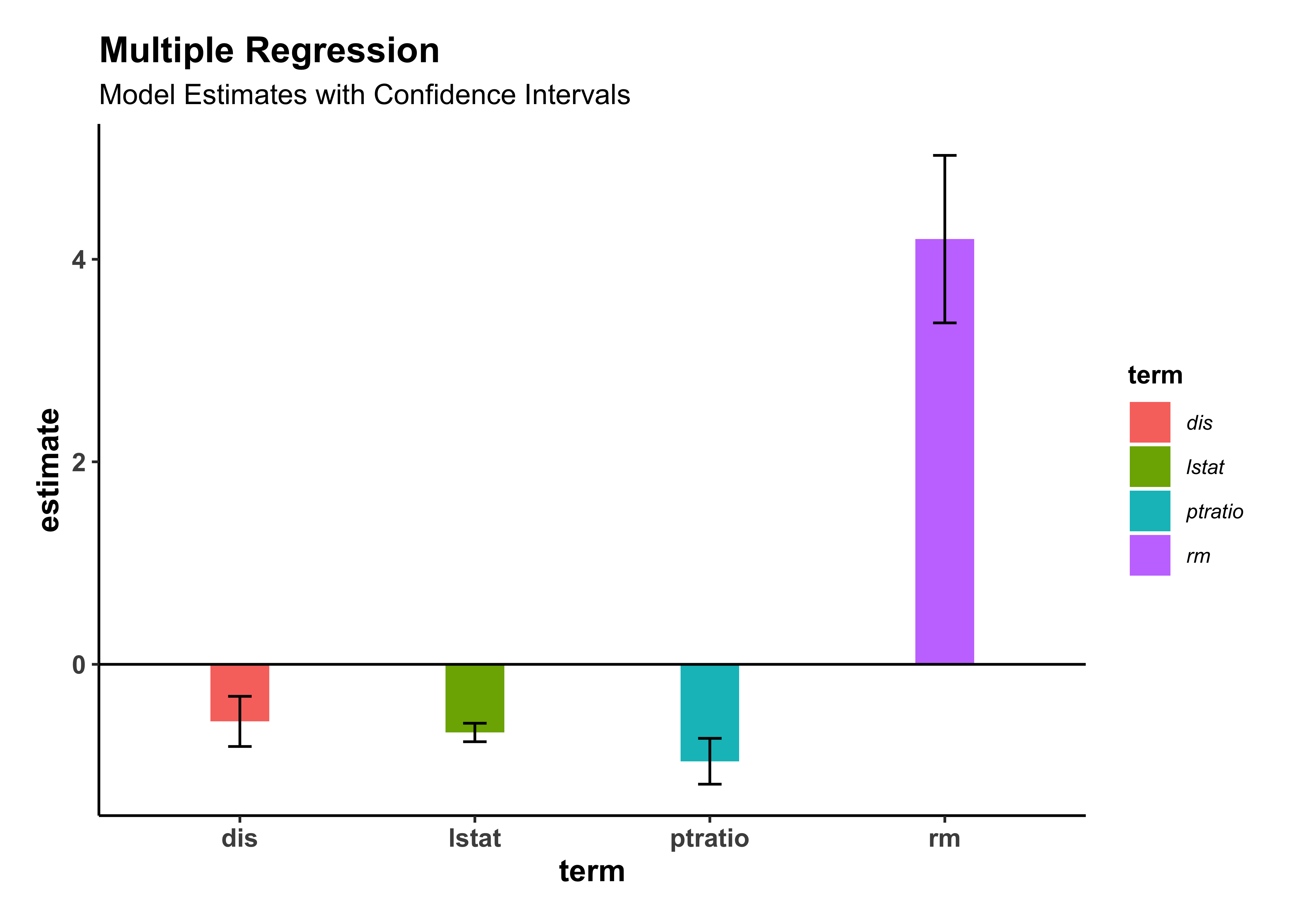

Our current best model can be stated as:

$\hat{c m e d v} \sim 24.459 - 0.563 * d i s - 0.673 * l s t a t - 0.957 * p t r a t i o + 4.199 * r m$

Workflow: Diagnostics

Let us use broom::augment to calculate residuals and predictions to arrive at a quick set of diagnostic plots.

housing_model_final_augment <- 
  housing_model_set %>% 
  filter(keep_vars == 4) %>% 
  
# augment the model
  mutate(augment_models =
           map(
             .x = models,
             .f = \(x) broom::augment(x)
           )) %>% 
  unnest(augment_models) %>% 
  select(cmedv:last_col())

housing_model_final_augment

ABCDEFGHIJ0123456789

cmedv <dbl>	lstat <dbl>	rm <dbl>	ptratio <dbl>	dis <dbl>	.fitted <dbl>	.resid <dbl>	.hat <dbl>	.sigma <dbl>	.cooksd <dbl>
24.0	4.98	6.58	15.3	4.09	31.767	-7.7666	0.00809	5.10	3.81e-03
21.6	9.14	6.42	17.8	4.97	25.433	-3.8328	0.00276	5.11	3.13e-04
34.7	4.03	7.18	17.8	4.97	32.080	2.6198	0.00596	5.11	3.18e-04
33.4	2.94	7.00	18.7	6.06	30.550	2.8501	0.00740	5.11	4.68e-04
36.2	5.33	7.15	18.7	6.06	29.567	6.6330	0.00747	5.10	2.56e-03
28.7	5.21	6.43	18.7	6.06	26.637	2.0630	0.00587	5.11	1.94e-04
22.9	12.43	6.01	15.2	5.56	23.655	-0.7554	0.00947	5.11	4.23e-05
22.1	19.15	6.17	15.2	5.95	19.585	2.5153	0.01679	5.11	8.44e-04
16.5	29.93	5.63	15.2	6.08	9.984	6.5165	0.04008	5.10	1.42e-02
18.9	17.10	6.00	15.2	6.59	19.897	-0.9974	0.01599	5.11	1.26e-04

housing_model_final_augment %>% 
  gf_point(.resid ~ .fitted, title = "Residuals vs Fitted") %>%
  gf_smooth() %>% 
  gf_theme(my_theme)
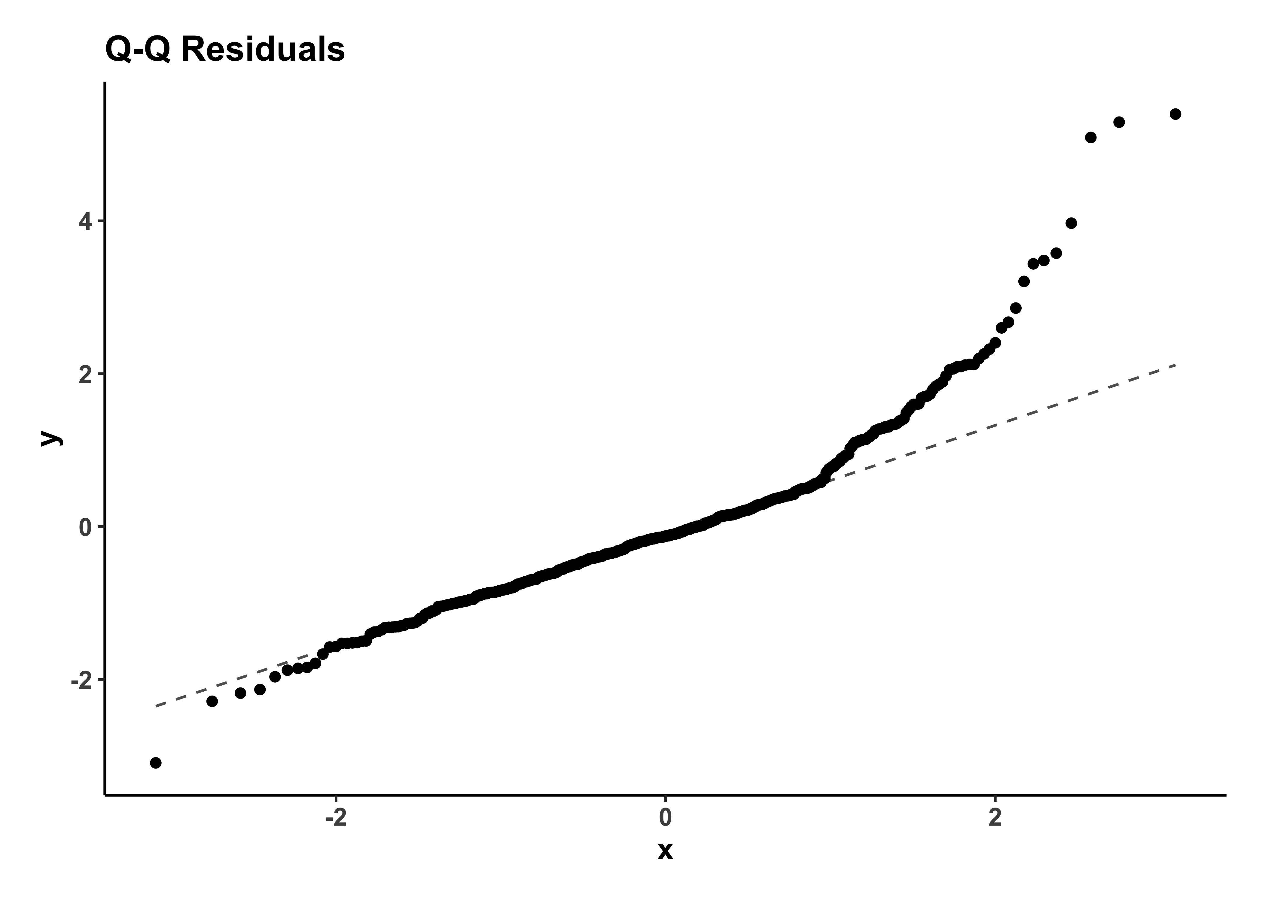
housing_model_final_augment %>% 
  gf_qq(~ .std.resid, title = "Q-Q Residuals") %>% 
  gf_qqline() %>%
  gf_theme(my_theme)
housing_model_final_augment %>% 
  gf_point(sqrt(.std.resid) ~ .fitted, 
           title = "Scale-Location Plot") %>%
    gf_smooth() %>% 
  gf_theme(my_theme)
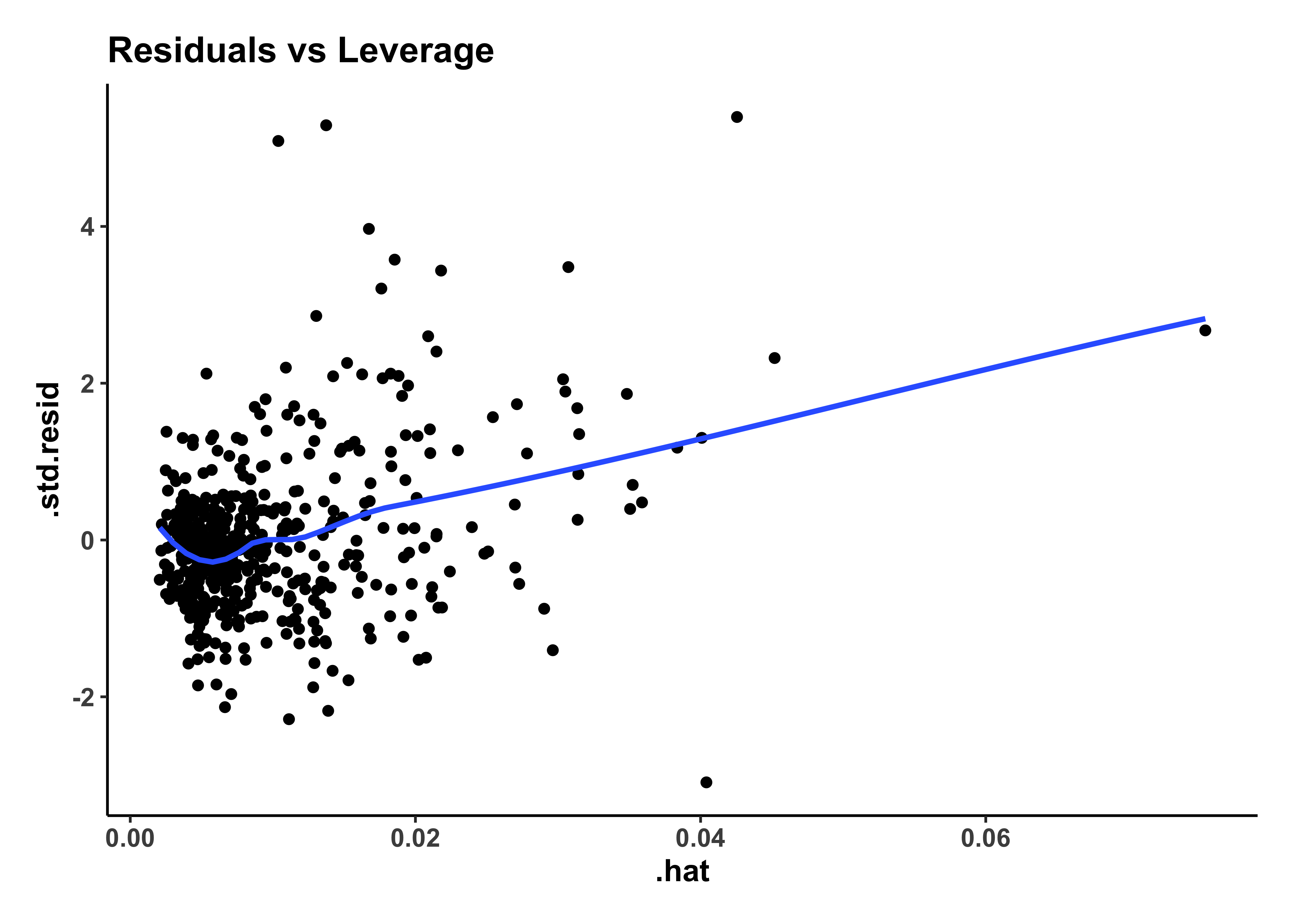
housing_model_final_augment %>% 
  gf_point(.std.resid ~ .hat, 
           title = "Residuals vs Leverage") %>%
    gf_smooth() %>% 
  gf_theme(my_theme)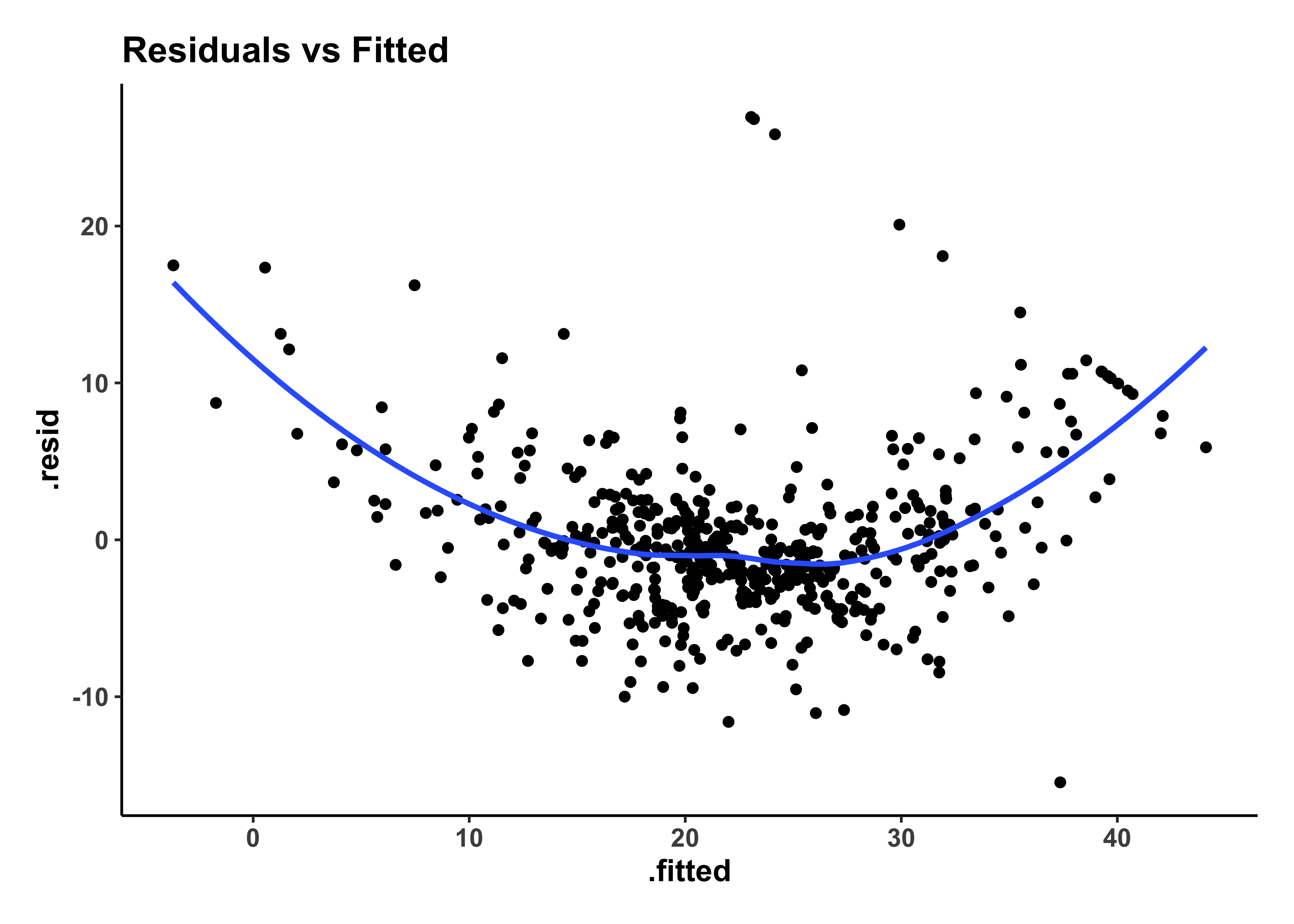

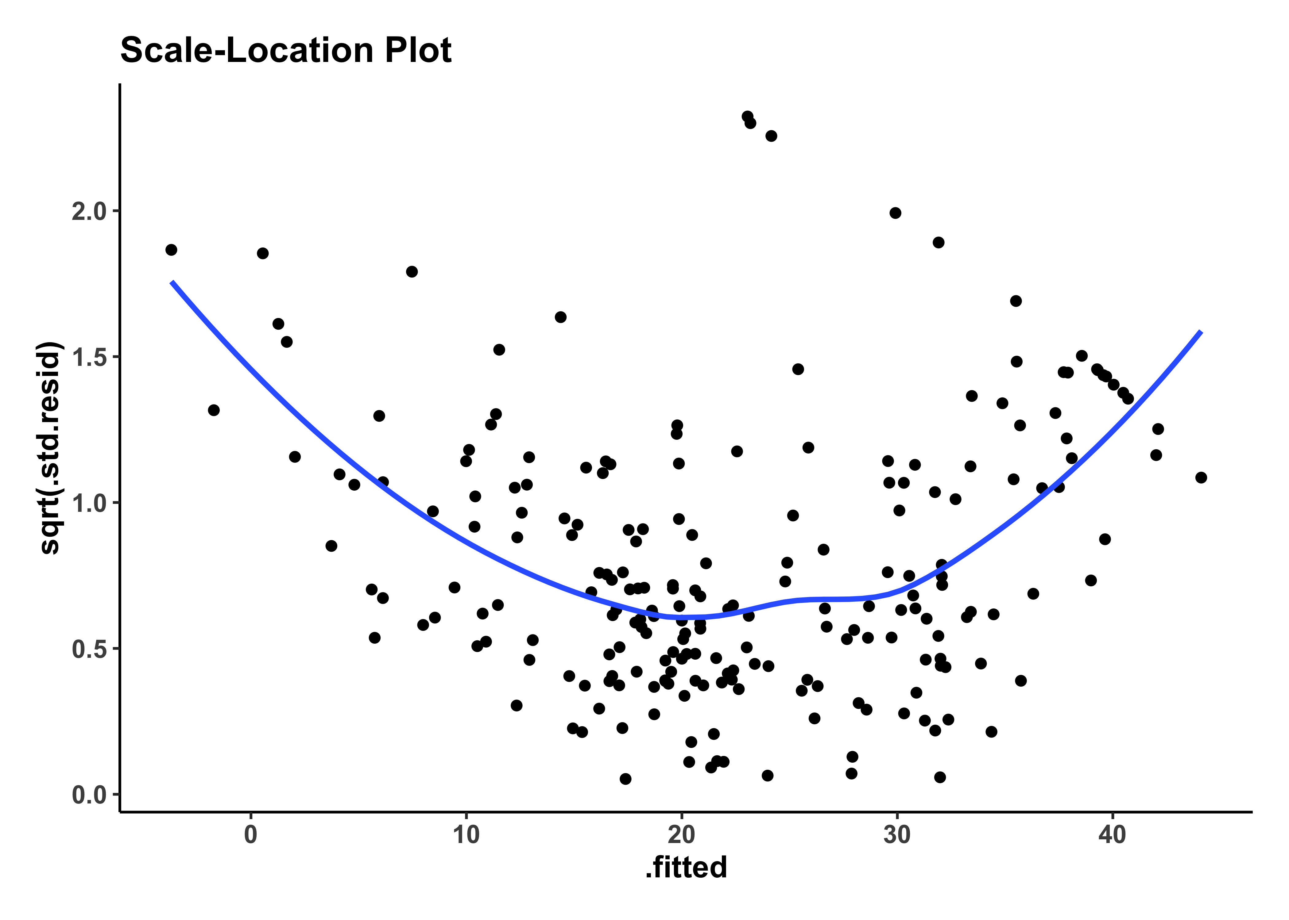
The residuals plot shows a curved trend, and certainly does not resemble the stars at night, so it is possible that we have left out some possible richness in our model-making, a “systemic inadequacy”.

The Q-Q plot of residuals also shows a J-shape which indicates a non-normal distribution of residuals.

These could indicate that more complex model ( e.g. linear model with interactions between variables ( i.e. product terms ) may be necessary.

Conclusion

We have used a multiple-regression workflow that takes all predictor variables into account in a linear model, and then systematically simplified that model such that the performance was just adequate.

The models we chose were all linear of course, but without interaction terms : each predictor was used only for its main effect. When the diagnostic plots were examined, we did see some shortcomings in the model. This could be overcome with a more complex model. These might include selected interactions, transformations of target( $c m e d v^{2}$ , or $s q r t (c m e d v)$ ) and some selected predictors.

References

James, Witten, Hastie, Tibshirani, An Introduction to Statistical Learning. Chapter 3. Linear Regression. https://hastie.su.domains/ISLR2/Labs/Rmarkdown_Notebooks/Ch3-linreg-lab.html

R Package Citations

Package	Version	Citation
corrgram	1.14	Wright (2021)
corrplot	0.92	Wei and Simko (2021)
GGally	2.2.1	Schloerke et al. (2024)
gt	0.10.1	Iannone et al. (2024)
infer	1.0.7	Couch et al. (2021)
ISLR	1.4	James et al. (2021)
janitor	2.2.0	Firke (2023)
reghelper	1.1.2	Hughes and Beiner (2023)

Couch, Simon P., Andrew P. Bray, Chester Ismay, Evgeni Chasnovski, Benjamin S. Baumer, and Mine Çetinkaya-Rundel. 2021. “infer: An R Package for Tidyverse-Friendly Statistical Inference.” Journal of Open Source Software 6 (65): 3661. https://doi.org/10.21105/joss.03661.

Firke, Sam. 2023. janitor: Simple Tools for Examining and Cleaning Dirty Data. https://CRAN.R-project.org/package=janitor.

Hughes, Jeffrey, and David Beiner. 2023. reghelper: Helper Functions for Regression Analysis. https://CRAN.R-project.org/package=reghelper.

Iannone, Richard, Joe Cheng, Barret Schloerke, Ellis Hughes, Alexandra Lauer, and JooYoung Seo. 2024. gt: Easily Create Presentation-Ready Display Tables. https://CRAN.R-project.org/package=gt.

James, Gareth, Daniela Witten, Trevor Hastie, and Rob Tibshirani. 2021. ISLR: Data for an Introduction to Statistical Learning with Applications in r. https://CRAN.R-project.org/package=ISLR.

Schloerke, Barret, Di Cook, Joseph Larmarange, Francois Briatte, Moritz Marbach, Edwin Thoen, Amos Elberg, and Jason Crowley. 2024. GGally: Extension to “ggplot2”. https://CRAN.R-project.org/package=GGally.

Wei, Taiyun, and Viliam Simko. 2021. R Package “corrplot”: Visualization of a Correlation Matrix. https://github.com/taiyun/corrplot.

Wright, Kevin. 2021. corrgram: Plot a Correlogram. https://CRAN.R-project.org/package=corrgram.

Footnotes

James, Witten, Hastie, Tibshirani,An Introduction to Statistical Learning. Chapter 3. Linear Regression https://hastie.su.domains/ISLR2/Labs/Rmarkdown_Notebooks/Ch3-linreg-lab.html ↩︎

Citation

BibTeX citation:

@online{v.2023,
  author = {V., Arvind},
  title = {Tutorial: {Multiple} {Linear} {Regression} with {Backward}
    {Selection}},
  date = {2023-05-03},
  url = {https://av-quarto.netlify.app/content/courses/Analytics/Modelling/Modules/LinReg/files/backward-selection-1.html},
  langid = {en},
  abstract = {Using Multiple Regression to predict Quantitative Target
    Variables}
}

For attribution, please cite this work as:

V., Arvind. 2023. “Tutorial: Multiple Linear Regression with Backward Selection.” May 3, 2023. https://av-quarto.netlify.app/content/courses/Analytics/Modelling/Modules/LinReg/files/backward-selection-1.html.