Playing with Leaflet

Author

Arvind Venkatadri

Published

May 13, 2017

Modified

July 29, 2025

Introduction

This Tutorial works through the ideas at Leaflet

Leaflet

Leaflet is a JavaScript library for creating dynamic maps that support panning and zooming along with various annotations like markers, polygons, and popups.

In this tutorial we will work only with vector data. In a second part, we will work with raster data in leaflet.

library(tidyverse)
library(leaflet)

# Data
library(osmdata) # Import OSM Vector Data into R

# devtools::install_github("datadotworld/data.world-r", build_vignettes = TRUE)
library(data.world)

Basic Features of a leaflet Map

# Set value for the minZoom and maxZoom settings.
# leaflet(options = leafletOptions(minZoom = 0, maxZoom = 18))

m <- leaflet() %>%
  # Add default OpenStreetMap map tiles
  addTiles() %>%
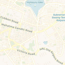
  # Set view to be roughly centred on Bangalore City
  setView(lng = 77.580643, lat = 12.972442, zoom = 12)

m

# Click on the map to zoom in; Shift+Click to zoom out

leaflet by default uses Open Street Map as its base map. We can use other base maps too, as we will see later.

Add Shapes to a Map

leaflet offers several commands to add points, markers, icons, lines, polylines and polygons to a map. Let us examine a few of these.

Add Markers with popups

m %>% addMarkers(
  lng = 77.580643, lat = 12.972442,
  popup = "The birthplace of Rvind"
)

# Click on the Marker for the popup to appear

This uses the default pin shape as the Marker.

Adding Popups to a Map

Popups are small boxes containing arbitrary HTML, that point to a specific point on the map. Use the addPopups() function to add standalone popup to the map.

m %>%
  addPopups(
    lng = 77.580643,
    lat = 12.972442,
    popup = paste(
      "The birthplace of Rvind",
      "<br>",
      "Website: <a href = https://arvindvenkatadri.com>Arvind V's Website </a>",
      "<br>"
    ),
    ## Ensuring we cannot close the popup,
    ## else we will not be able to find where it is,
    ## since there is no Marker

    options = popupOptions(closeButton = FALSE)
  )

Popups are usually added to icons, Markers and other shapes can show up when these are clicked.

Adding Labels to a Map

Labels are messages attached to all shapes, using the argument label wherever it is available.

Labels are static, and Popups are usually visible on mouse click. Hence a Marker can have both a label and a popup. For example, the function addPopup() offers only a popup argument, whereas the function addMarkers() offers both a popup and a label argument.

It is also possible to create labels standalone using addLabelOnlyMarkers() where we can show only text and no Markers.

m %>%
  addMarkers(
    lng = 77.580643,
    lat = 12.972442,

    # Here is the Label defn.
    label = "The birthplace of Rvind",
    labelOptions = labelOptions(
      noHide = TRUE, # Label always visible
      textOnly = F,
      textsize = 20
    ),

    # And here is the popup defn.
    popup = paste(
      "PopUp Text: <a href = https://arvindvenkatadri.com>Arvind V's Website </a>",
      "<br>"
    )
  )

Adding Circles and CircleMarkers on a Map

We can add shapes on to a map to depict areas or locations of interest.

addCircles and addCircleMarkers

The radius argument works differently in addCircles() and addCircleMarkers().

# Some Cities in the US and their location
md_cities <- tibble(
  name = c("Baltimore", "Frederick", "Rockville", "Gaithersburg", "Bowie", "Hagerstown", "Annapolis", "College Park", "Salisbury", "Laurel"),
  pop = c(619493, 66169, 62334, 61045, 55232, 39890, 38880, 30587, 30484, 25346),
  lat = c(39.2920592, 39.4143921, 39.0840, 39.1434, 39.0068, 39.6418, 38.9784, 38.9897, 38.3607, 39.0993),
  lng = c(-76.6077852, -77.4204875, -77.1528, -77.2014, -76.7791, -77.7200, -76.4922, -76.9378, -75.5994, -76.8483)
)


md_cities %>%
  leaflet() %>%
  addTiles() %>%
  # CircleMarkers, in blue
  # radius scales the Marker. Units are in Pixels!!
  # Here, radius is made proportional to `pop` number
  addCircleMarkers(
    radius = ~ pop / 1000, # Pixels!!
    color = "blue",
    stroke = FALSE, # no border for the Markers
    opacity = 0.8
  ) %>%
  # Circles, in red
  addCircles(
    radius = 5000, # Meters !!!
    stroke = TRUE,
    color = "yellow", # Stroke Colour
    weight = 3, # Stroke Weight
    fill = TRUE,
    fillColor = "red",
  )

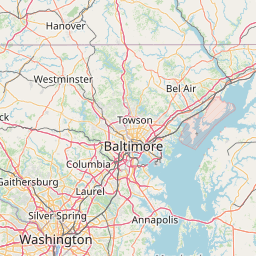
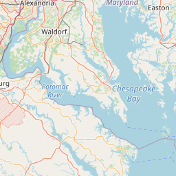
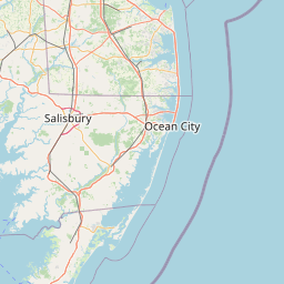
The shapes need not be of fixed size or colour; their attributes can be made to correspond to other attribute variables in the geospatial data, as we did with radius in the addCircleMarkers() function above.

Adding Rectangles to a Map

## Adding Rectangles
leaflet() %>%
  addTiles() %>%
  setView(lng = 77.580643, lat = 12.972442, zoom = 6) %>%
  addRectangles(
    lat1 = 10.3858, lng1 = 75.0595,
    lat2 = 12.8890, lng2 = 77.9625
  )

Add Polygons to a Map

## Adding Polygons
leaflet() %>%
  addTiles() %>%
  setView(lng = 77.580643, lat = 12.972442, zoom = 6) %>%
  # arbitrary vector data for lat and lng
  addPolygons(
    lng = c(73.5, 75.9, 76.1, 77.23, 79.8),
    lat = c(10.12, 11.04, 11.87, 12.04, 10.7)
  )

Add PolyLines to a Map

This can be useful say for manually marking a route on a map, with waypoints.

leaflet() %>%
  addTiles() %>%
  setView(lng = 77.580643, lat = 12.972442, zoom = 6) %>%
  # arbitrary vector data for lat and lng
  # If start and end points are the same, it looks like Polygon
  # Without the fill
  # Two Vectors
  addPolylines(
    lng = c(73.5, 75.9, 76.1, 77.23, 79.8),
    lat = c(10.12, 11.04, 11.87, 12.04, 10.7)
  ) %>%
  # Add Waypoint Icons
  # Same Two Vectors
  addMarkers(
    lng = c(73.5, 75.9, 76.1, 77.23, 79.8),
    lat = c(10.12, 11.04, 11.87, 12.04, 10.7)
  )

As seen, we have created Markers, Labels, Polygons, and PolyLines using fixed.i.e. literal text and numbers. In the following we will also see how external geospatial data columns can be used instead of these literals.

The mapedit package

https://r-spatial.org//r/2017/01/30/mapedit_intro.html can also be used to interactively add shapes onto a map and save as an geo-spatial object.

Using `leaflet` with External Geospatial Data

On to something more complex. We want to plot an external user-defined set of locations on a leaflet map. leaflet takes in geographical data in many ways and we will explore most of them.

POINT Data Sources for `leaflet`

Point data for markers can come from a variety of sources:

Vectors: Simply provide numeric vectors as lng and lat arguments, which we have covered already in the preceding sections.
Matrices: Two-column numeric matrices (first column is longitude, second is latitude)
Data Frames: Data frame/tibble with latitude and longitude columns. You can explicitly tell the marker function which columns contain the coordinate data (e.g. addMarkers(lng = ~Longitude, lat = ~Latitude)), or let the function look for columns named lat/latitude and lon/lng/long/longitude (case insensitive).
Package sp” SpatialPoints or SpatialPointsDataFrame objects (from the sp package)
Package sf: POINT,sfc_POINT, andsfobjects (from thesf` package); only X and Y dimensions will be considered

Not using sp

We will not consider the use of sp related data structures for plotting POINTs in leaflet since sp is being phased out in favour of the more modern package sf.

Points using simple Data Frames

Let us read in the data set from data.world that gives us POINT locations of all airports in India in a data frame / tibble. The dataset is available at https://query.data.world/s/ahtyvnm2ybylf65syp4rsb5tulxe6a and, for poor peasants especially, also by clicking the download button below. Save it in a convenient data folder in your project and read it in.

Using data.world

You will need the package data.world and also need to register your credentials for that page with RStudio. The (simple!) instructions are available here at data.world.

ABCDEFGHIJ0123456789

id <int>	ident <chr>	type <chr>	name <chr>	lat <dbl>	lon <dbl>	elevation_ft <int>	continent <chr>	iso_country <chr>	iso_region <chr>
26555	VIDP	large_airport	Indira Gandhi International Airport	28.56650	77.1031	777	AS	IN	IN-DL
26434	VABB	large_airport	Chhatrapati Shivaji International Airport	19.08870	72.8679	39	AS	IN	IN-MM
35145	VOBL	large_airport	Kempegowda International Airport	13.19790	77.7063	3000	AS	IN	IN-KA
26618	VOMM	large_airport	Chennai International Airport	12.99001	80.1693	52	AS	IN	IN-TN
26444	VAGO	large_airport	Dabolim Airport	15.38080	73.8314	150	AS	IN	IN-GA
26609	VOCI	large_airport	Cochin International Airport	10.15200	76.4019	30	AS	IN	IN-KL

Here is the data:

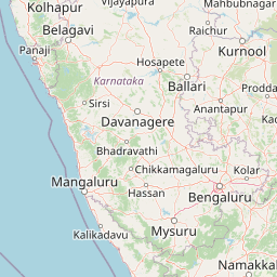
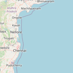
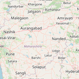
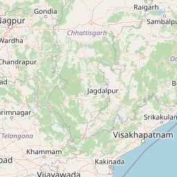
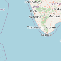
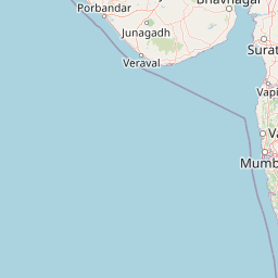
Let us plot this in leaflet, using an ESRI National Geographic style map instead of the default OSM Base Map. We will also place small circle markers for each airport.

leaflet(data = india_airports) %>%
  setView(lat = 18, lng = 77, zoom = 4) %>%
  # Add NatGeo style base map
  addProviderTiles(providers$Esri.NatGeoWorldMap) %>% # ESRI Basemap

  # Add Markers for each airport
  addCircleMarkers(
    lng = ~lon, lat = ~lat,
    # Optional, variables stated for clarity
    # leaflet can automatically detect lon-lat columns
    # if they are appropriately named in the data
    # longitude/lon/lng
    # latitude/lat
    radius = 2, # Pixels
    color = "red",
    opacity = 1
  )

We can also change the icon for each airport. Let us try one of the several icon families that we can use with leaflet : glyphicons, ionicons, and fontawesome icons. Here is the IATA icon: download and save it and make sure this code below has the proper path to this .png file!

IATA Logo

# Define popup message for each airport
# Based on data in india_airports
popup <- paste(
  "<strong>",
  india_airports$name,
  "</strong><br>",
  india_airports$iata_code,
  "<br>",
  india_airports$municipality,
  "<br>",
  "Elevation(feet)",
  india_airports$elevation_ft,
  "<br>",
  india_airports$wikipedia_link,
  "<br>"
)

iata_icon <- makeIcon(
  "images/iata-logo-transp.png", # Downloaded from www.iata.org
  iconWidth = 24,
  iconHeight = 24,
  iconAnchorX = 0,
  iconAnchorY = 0
)

# Create the Leaflet map
leaflet(data = india_airports) %>%
  setView(lat = 18, lng = 77, zoom = 4) %>%
  addProviderTiles(providers$Esri.NatGeoWorldMap) %>%
  addMarkers(
    icon = iata_icon,
    popup = popup
  )

There are other icons we can use to mark the POINTs. leaflet allows the use of ionicons, glyphicons, and FontAwesomeIcons.

It is possible to create a list of icons, so that different Markers can have different icons. Let us try to map the MNCs in the ITPL area of Bangalore: we use the ideas in Using Leaflet Markers @JLA-Data.net

# Make a dataframe of addresses of Companies we wan to plot in ITPL
companies_itpl <-
  data.frame(
    ticker = c(
      "MBRDI",
      "DTICI",
      "IBM",
      "Exxon",
      "Mindtree",
      "FIS Global",
      "Sasken",
      "LTI"
    ),
    lat = c(
      12.986178620989264,
      12.984160906190121,
      12.983659088566357,
      12.985112265986636,
      12.983794997606187,
      12.980658616215155,
      12.982080447350246,
      12.981338168875348
    ),
    lon = c(
      77.7270652183105,
      77.72808445774321,
      77.73103488768001,
      77.72935046040699,
      77.7227844126931,
      77.72685064158782,
      77.72545589289041,
      77.72287024338216
    )
  ) %>% sf::st_as_sf(coords = c("lon", "lat"), crs = 4326)

# Vanilla leaflet map
leaflet(companies_itpl) %>%
  addTiles() %>%
  addMarkers()

Points using `sf` objects

We will use data from an sf data object. This differs from the earlier situation where we had a simple data frame with lon and lat columns. In sf, as we know, the lon and lat info is embedded in the geometry column of the sf data frame.

The tmap package has a data set of all World metro cities, titled metro. We will plot these on the map and also scale the markers in proportion to one of the feature attributes, pop2030. The popup will be the name of the metro city. We will also use the CartoDB.Positron base map.

Note that the metro data set has a POINT geometry, as needed!

data(metro, package = "tmap")
metro

ABCDEFGHIJ0123456789

	name <chr>	name_long <chr>	iso_a3 <chr>	pop1950 <dbl>	pop1960 <dbl>	pop1970 <dbl>	pop1980 <dbl>	pop1990 <dbl>	pop2000 <dbl>
2	Kabul	Kabul	AFG	170784	285352	471891	977824	1549320	2401109
8	Algiers	El Djazair (Algiers)	DZA	516450	871636	1281127	1621442	1797068	2140577
13	Luanda	Luanda	AGO	138413	219427	459225	771349	1390240	2591388
16	Buenos Aires	Buenos Aires	ARG	5097612	6597634	8104621	9422362	10513284	12406780
17	Cordoba	Cordoba	ARG	429249	605309	809794	1009521	1200168	1347561
25	Rosario	Rosario	ARG	554483	671349	816230	953491	1083819	1152387
32	Yerevan	Yerevan	ARM	341432	537759	778158	1041587	1174524	1111301
33	Adelaide	Adelaide	AUS	429277	571822	850168	971856	1081618	1141623
34	Brisbane	Brisbane	AUS	441718	602999	904777	1134833	1381306	1666203
37	Melbourne	Melbourne	AUS	1331966	1851220	2499109	2839019	3154314	3460541

leaflet(data = metro) %>%
  setView(lat = 18, lng = 77, zoom = 4) %>%
  # Add CartoDB.Positron
  addProviderTiles(providers$CartoDB.Positron) %>% # CartoDB Basemap

  # Add Markers for each airport
  addCircleMarkers(
    radius = ~ sqrt(pop2030) / 350,
    color = "red",
    popup = paste(
      "Name: ", metro$name, "<br>",
      "Population 2030: ", metro$pop2030
    )
  )

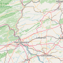
We can also try downloading an sf data frame with POINT geometry from say OSM data https://www.openstreetmap.org/#map=16/12.9766/77.5888. Let us get hold of restaurants data in Malleswaram, Bangalore from OSM data:

bbox <- osmdata::getbb("Malleswaram, Bengaluru")
bbox

       min      max
x 77.55033 77.59033
y 12.98274 13.02274

locations <-
  osmdata::opq(bbox = bbox) %>%
  osmdata::add_osm_feature(key = "amenity", value = "restaurant") %>%
  osmdata_sf() %>%
  purrr::pluck("osm_points") %>%
  dplyr::select(name, cuisine, geometry) %>%
  dplyr::filter(cuisine == "indian")

locations %>% head()

ABCDEFGHIJ0123456789

	name <chr>	cuisine <chr>	geometry <sf_POINT>
461539222	Adiga's	indian	<sf_POINT>
598500940	Udupi Sri Krishnarajathadri	indian	<sf_POINT>
673377213	Sana Di Ge	indian	<sf_POINT>
673860152	New Shanthi Sagar	indian	<sf_POINT>
1116484556	Kabab Studio	indian	<sf_POINT>
1448082496	Sai Shakti	indian	<sf_POINT>

# Fontawesome icons seem to work in `leaflet` only up to FontAwesome V4.7.0.
# The Fontawesome V4.7.0 Cheatsheet is here: <https://fontawesome.com/v4/cheatsheet/>


leaflet(
  data = locations,
  options = leafletOptions(minZoom = 12)
) %>%
  addProviderTiles(providers$CartoDB.Voyager) %>%
  # Regular `leaflet` code
  addAwesomeMarkers(
    icon = awesomeIcons(
      icon = "fa-coffee",
      library = "fa",
      markerColor = "blue",
      iconColor = "black",
      iconRotate = TRUE
    ),
    popup = paste(
      "Name: ", locations$name, "<br>",
      "Food: ", locations$cuisine
    )
  )

Fontawesome Workaround**

For more later versions of Fontawesome, here below is a workaround from https://github.com/rstudio/leaflet/issues/691. Despite this some fontawesome icons simply do not seem to show up. Aiyooo….;-()

( Update Dec 2023: Seems OK now…)

library(fontawesome)
coffee <- makeAwesomeIcon(
  text = fa("mug-hot"), # mug-hot was introduced in fa version 5
  iconColor = "black",
  markerColor = "blue",
  library = "fa"
)


leaflet(data = locations) %>%
  addProviderTiles(providers$CartoDB.Voyager) %>%
  # Workaround code

  addAwesomeMarkers(
    icon = coffee,
    popup = paste(
      "Name: ", locations$name, "<br>",
      "Food: ", locations$cuisine, "<br>"
    )
  )

leaflet detects sf POINT geometry

Note that leaflet automatically detects the lon/lat columns from within the POINT geometry column of the sf data frame.

Points using Two-Column Matrices

We can now quickly try providing lon and lat info in a two column matrix.This can be useful to plot a bunch of points recorded on a mobile phone app.

mysore5 <- matrix(
  c(
    runif(5, 76.652985 - 0.01, 76.652985 + 0.01),
    runif(5, 12.311827 - 0.01, 12.311827 + 0.01)
  ),
  nrow = 5
)
mysore5

         [,1]     [,2]
[1,] 76.64561 12.30481
[2,] 76.64341 12.30308
[3,] 76.64324 12.31361
[4,] 76.64518 12.31857
[5,] 76.64842 12.31452

leaflet(data = mysore5) %>%
  addProviderTiles(providers$OpenStreetMap) %>%
  # Pick an icon from <https://www.w3schools.com/bootstrap/bootstrap_ref_comp_glyphs.asp>
  addAwesomeMarkers(
    icon = awesomeIcons(
      icon = "music",
      iconColor = "black",
      library = "glyphicon"
    ),
    popup = "Carnatic Music !!"
  )

Polygons, Lines, and Polylines Data Sources for `leaflet`

We have seen how to get POINT data into leaflet.

LINE and POLYGON data can also come from a variety of sources:

sf package: MULTIPOLYGON, POLYGON, MULTILINESTRING, and LINESTRING objects (from the sf package)
sp package: SpatialPolygons, SpatialPolygonsDataFrame, Polygons, and Polygon objects (from the sp package)
~~**sp package:SpatialLines, SpatialLinesDataFrame, Lines, and Line objects (from the sp package)~~
maps package:map objects (from the maps package’s map() function); use map(fill = TRUE) for polygons, FALSE for polylines
Matrices:Two-column numeric matrix; the first column is longitude and the second is latitude. Polygons are separated by rows of (NA, NA). It is not possible to represent multi-polygons nor polygons with holes using this method; Sounds very clumsy and better not attempt. Use sf instead.

We will concentrate on using sf data into leaflet. We may explore maps() objects at a later date.

Polygons/MultiPolygons and LineString/MultiLineString using `sf` data frames

Let us download College buildings, parks, and the cycling lanes in Amsterdam, Netherlands, and plot these in leaflet.

library(osmdata)
# Option 1
# Gives too large a bbox
bbox <- osmdata::getbb("Amsterdam, Netherlands")
# bbox

# Setting bbox manually is better
amsterdam_coords <- matrix(c(4.85, 4.95, 52.325, 52.375),
  byrow = TRUE,
  nrow = 2, ncol = 2,
  dimnames = list(c("x", "y"), c("min", "max"))
)
amsterdam_coords

     min    max
x  4.850  4.950
y 52.325 52.375

colleges <- amsterdam_coords %>%
  osmdata::opq() %>%
  osmdata::add_osm_feature(
    key = "amenity",
    value = "college"
  ) %>%
  osmdata_sf() %>%
  purrr::pluck("osm_polygons")

parks <- amsterdam_coords %>%
  osmdata::opq() %>%
  osmdata::add_osm_feature(key = "landuse", value = "grass") %>%
  osmdata_sf() %>%
  purrr::pluck("osm_polygons")

roads <- amsterdam_coords %>%
  osmdata::opq() %>%
  osmdata::add_osm_feature(
    key = "highway",
    value = "primary"
  ) %>%
  osmdata_sf() %>%
  purrr::pluck("osm_lines")

cyclelanes <- amsterdam_coords %>%
  osmdata::opq() %>%
  osmdata::add_osm_feature(key = "cycleway") %>%
  osmdata_sf() %>%
  purrr::pluck("osm_lines")

We have 12 colleges, 3371 parks, 309 roads, and 281 cycle lanes in our data.

leaflet() %>%
  addTiles() %>%
  addPolygons(
    data = colleges, color = "yellow",
    popup = ~ colleges$name
  ) %>%
  addPolygons(data = parks, color = "seagreen", popup = parks$name) %>%
  addPolylines(data = roads, color = "red") %>%
  addPolylines(data = cyclelanes, color = "purple")

Using Raster Data in `leaflet`[Work in Progress!]

So far all the geospatial data we have plotted in leaflet has been vector data.

We will now explore how to plot raster data using leaflet. Raster data are used to depict continuous variables across space, such as vegetation, salinity, forest cover etc. Satellite imagery is frequently available as raster data.

Importing Raster Data [Work in Progress!]

Raster data can be imported into R in many ways:

using the maptiles package
using the OpenStreetMap package

library(terra)
library(maptiles)
# library(OpenStreetMap) # causes RStudio to crash...

Bells and Whistles in `leaflet`: layers, groups, legends, and graticules

Adding Legends

## Generate some random lat lon data around Bangalore
df <- tibble(
  lat = runif(20, min = 11.97, max = 13.07),
  lng = runif(20, min = 77.48, max = 77.68),
  col = sample(c("red", "blue", "green"), 20,
    replace = TRUE
  ),
  stringsAsFactors = FALSE
)

df %>%
  leaflet() %>%
  addTiles() %>%
  addCircleMarkers(color = df$col) %>%
  addLegend(values = df$col, labels = LETTERS[1:3], colors = c("blue", "red", "green"))

Using Web Map Services (WMS) [Work in Progress!]

To be included.

Introduction

Basic Features of a leaflet Map

Add Shapes to a Map

Add Markers with popups

Adding Popups to a Map

Adding Labels to a Map

Adding Circles and CircleMarkers on a Map

Adding Rectangles to a Map

Add Polygons to a Map

Add PolyLines to a Map

Using leaflet with External Geospatial Data

POINT Data Sources for leaflet

Points using simple Data Frames

Points using sf objects

Points using Two-Column Matrices

Polygons, Lines, and Polylines Data Sources for leaflet

Polygons/MultiPolygons and LineString/MultiLineString using sf data frames

Using Raster Data in leaflet[Work in Progress!]

Importing Raster Data [Work in Progress!]

Bells and Whistles in leaflet: layers, groups, legends, and graticules

Adding Legends

Using Web Map Services (WMS) [Work in Progress!]

Using `leaflet` with External Geospatial Data

POINT Data Sources for `leaflet`

Points using `sf` objects

Polygons, Lines, and Polylines Data Sources for `leaflet`

Polygons/MultiPolygons and LineString/MultiLineString using `sf` data frames

Using Raster Data in `leaflet`[Work in Progress!]

Bells and Whistles in `leaflet`: layers, groups, legends, and graticules