Antarctic Sea ice

Setting up R Packages

library(tidyverse)
library(mosaic)
library(skimr)
library(ggformula)

Plot Theme

Show the Code

# https://stackoverflow.com/questions/74491138/ggplot-custom-fonts-not-working-in-quarto

# Chunk options
knitr::opts_chunk$set(
  fig.width = 7,
  fig.asp = 0.618, # Golden Ratio
  # out.width = "80%",
  fig.align = "center"
)
### Ggplot Theme
### https://rpubs.com/mclaire19/ggplot2-custom-themes

theme_custom <- function() {
  font <- "Roboto Condensed" # assign font family up front

  theme_classic(base_size = 14) %+replace% # replace elements we want to change

    theme(
      panel.grid.minor = element_blank(), # strip minor gridlines
      text = element_text(family = font),
      # text elements
      plot.title = element_text( # title
        family = font, # set font family
        size = 20, # set font size
        face = "bold", # bold typeface
        hjust = 0, # left align
        # vjust = 2                #raise slightly
        margin = margin(0, 0, 10, 0)
      ),
      plot.subtitle = element_text( # subtitle
        family = font, # font family
        size = 14, # font size
        hjust = 0,
        margin = margin(2, 0, 5, 0)
      ),
      plot.caption = element_text( # caption
        family = font, # font family
        size = 8, # font size
        hjust = 1
      ), # right align

      axis.title = element_text( # axis titles
        family = font, # font family
        size = 10 # font size
      ),
      axis.text = element_text( # axis text
        family = font, # axis family
        size = 8
      ) # font size
    )
}

# Set graph theme
theme_set(new = theme_custom())
#

Introduction

The extent of Antarctic Sea Ice over time is monitored by the National Snow and Ice Data Center https://nsidc.org/.

Read the Data

Excel Data

The data is an excel sheet. Inspect it first in Excel and decide which sheet you need, and which part of the data you need. There are multiple sheets! Then use readxl::read_xlsx(..) to read it into R. NOTE: The sheet that contains our data of interest is titled “SH-Daily-Extent”.

Inspect the Data

ABCDEFGHIJ0123456789

...1 <chr>	...2 <dbl>	1978 <dbl>	1979 <dbl>	1980 <dbl>	1981 <dbl>	1982 <dbl>	1983 <dbl>	1984 <dbl>	1985 <dbl>
January	1	NA	NA	5.967	6.323	NA	6.508	NA	NA
NA	2	NA	6.945	NA	NA	7.039	NA	6.944	6.527
NA	3	NA	NA	5.674	5.791	NA	6.170	NA	NA
NA	4	NA	6.838	NA	NA	6.689	NA	6.653	6.061
NA	5	NA	NA	5.584	5.351	NA	5.869	NA	NA
NA	6	NA	6.638	NA	NA	6.393	NA	6.296	5.665
NA	7	NA	NA	5.329	5.191	NA	5.660	NA	NA
NA	8	NA	6.270	NA	NA	6.084	NA	5.935	5.310
NA	9	NA	NA	5.000	4.775	NA	5.305	NA	NA
NA	10	NA	6.138	NA	NA	5.862	NA	5.629	4.934

Appreciate the structure of this data. You may even want to open it in Excel for a closer look. List any imperfections in your Data Dictionary. Why do these matter now? Why might they not have mattered earlier, up to now?

Data Dictionary

Quantitative Variables

Write in.

Qualitative Variables

Write in.

Observations

Write in.

Analyse/Transform the Data

Try to figure what may be needed, based on the imperfections noted above, what you may attempt to clean the data. Refer to your “list of imperfections” in the data.

Then look at the code below and execute line by line to get an idea.

```{r}
#| label: data-preprocessing
#
# Write in your code here
# to prepare this data as shown below
# to generate the plot that follows
```

Show the Code

ice %>%
  # Select columns
  # Rename some while selecting !!
  select("month" = ...1, "day" = ...2, c(4:49)) %>%
  # Fill the month column! Yes!!
  tidyr::fill(month) %>%
  # Make Wide Data into Long
  pivot_longer(
    cols = -c(month, day),
    names_to = "series",
    values_to = "values"
  ) %>%
  # Regular Munging
  mutate(
    series = as.integer(series),
    month = factor(month,
      levels = month.name,
      labels = month.name,
      ordered = TRUE
    ),
    # Note munging for date!!
    # Using the lubridate package, part of tidyverse
    date = lubridate::make_date(
      year = series,
      month = month,
      day = day
    )
  ) -> ice_prepared

ice_prepared

ABCDEFGHIJ0123456789

month <ord>	day <dbl>	series <int>	values <dbl>	date <date>
January	1	1979	NA	1979-01-01
January	1	1980	5.967	1980-01-01
January	1	1981	6.323	1981-01-01
January	1	1982	NA	1982-01-01
January	1	1983	6.508	1983-01-01
January	1	1984	NA	1984-01-01
January	1	1985	NA	1985-01-01
January	1	1986	7.718	1986-01-01
January	1	1987	NA	1987-01-01
January	1	1988	NA	1988-01-01

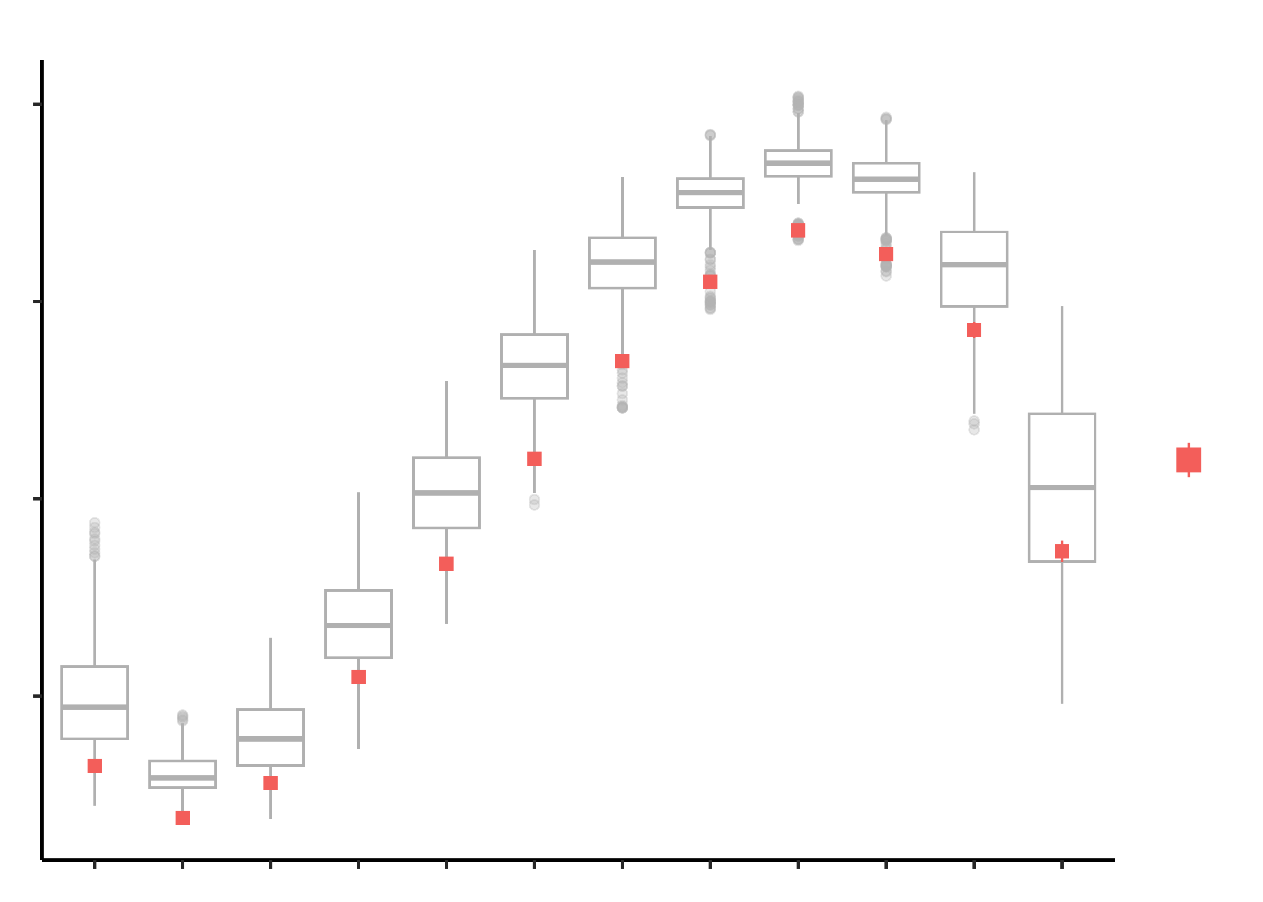
Research Question

Note

Write in! Look first at the graph!

Plot the Data

Tasks and Discussion

Complete the Data Dictionary.
Select and Transform the variables as shown.
Create the graphs shown and discuss the following questions:
- Identify the type of charts
- Identify the variables used for various geometrical aspects (x, y, fill…). Name the variables appropriately.
- What research activity might have been carried out to obtain the data graphed here? Provide some details.
- What might have been the Hypothesis/Research Question to which the response was Chart?
- What might the red points represent?
- What is perhaps a befuddling aspect of this graph until you…Ohhh!!!!!!
- Draw a sketch of a similar chart for ice extents in the Arctic.