Happy Families are All Alike
Slides and Tutorials
“No matter what happens in life, be good to people. Being good to people is a wonderful legacy to leave behind.”
— Taylor Swift
Plot Fonts and Theme
Show the Code
library(systemfonts)
library(showtext)
## Clean the slate
systemfonts::clear_local_fonts()
systemfonts::clear_registry()
##
showtext_opts(dpi = 96) # set DPI for showtext
sysfonts::font_add(
family = "Alegreya",
regular = "../../../../../../fonts/Alegreya-Regular.ttf",
bold = "../../../../../../fonts/Alegreya-Bold.ttf",
italic = "../../../../../../fonts/Alegreya-Italic.ttf",
bolditalic = "../../../../../../fonts/Alegreya-BoldItalic.ttf"
)Error in check_font_path(bold, "bold"): font file not found for 'bold' typeShow the Code
sysfonts::font_add(
family = "Roboto Condensed",
regular = "../../../../../../fonts/RobotoCondensed-Regular.ttf",
bold = "../../../../../../fonts/RobotoCondensed-Bold.ttf",
italic = "../../../../../../fonts/RobotoCondensed-Italic.ttf",
bolditalic = "../../../../../../fonts/RobotoCondensed-BoldItalic.ttf"
)
showtext_auto(enable = TRUE) # enable showtext
##
theme_custom <- function() {
font <- "Alegreya" # assign font family up front
theme_classic(base_size = 14, base_family = font) %+replace% # replace elements we want to change
theme(
text = element_text(family = font), # set base font family
# text elements
plot.title = element_text( # title
family = font, # set font family
size = 24, # set font size
face = "bold", # bold typeface
hjust = 0, # left align
margin = margin(t = 5, r = 0, b = 5, l = 0)
), # margin
plot.title.position = "plot",
plot.subtitle = element_text( # subtitle
family = font, # font family
size = 14, # font size
hjust = 0, # left align
margin = margin(t = 5, r = 0, b = 10, l = 0)
), # margin
plot.caption = element_text( # caption
family = font, # font family
size = 9, # font size
hjust = 1
), # right align
plot.caption.position = "plot", # right align
axis.title = element_text( # axis titles
family = "Roboto Condensed", # font family
size = 12
), # font size
axis.text = element_text( # axis text
family = "Roboto Condensed", # font family
size = 9
), # font size
axis.text.x = element_text( # margin for axis text
margin = margin(5, b = 10)
)
# since the legend often requires manual tweaking
# based on plot content, don't define it here
)
}Show the Code
```{r}
#| cache: false
#| code-fold: true
## Set the theme
theme_set(new = theme_custom())
## Use available fonts in ggplot text geoms too!
update_geom_defaults(geom = "text", new = list(
family = "Roboto Condensed",
face = "plain",
size = 3.5,
color = "#2b2b2b"
))
```
| Variable #1 | Variable #2 | Chart Names | Chart Shape | |
|---|---|---|---|---|
| Qual | None | Bar Chart |
| No | Pronoun | Answer | Variable/Scale | Example | What Operations? |
|---|---|---|---|---|---|
| 3 | How, What Kind, What Sort | A Manner / Method, Type or Attribute from a list, with list items in some " order" ( e.g. good, better, improved, best..) | Qualitative/Ordinal | Socioeconomic status (Low income, Middle income, High income),Education level (HighSchool, BS, MS, PhD),Satisfaction rating(Very much Dislike, Dislike, Neutral, Like, Very Much Like) | Median,Percentile |
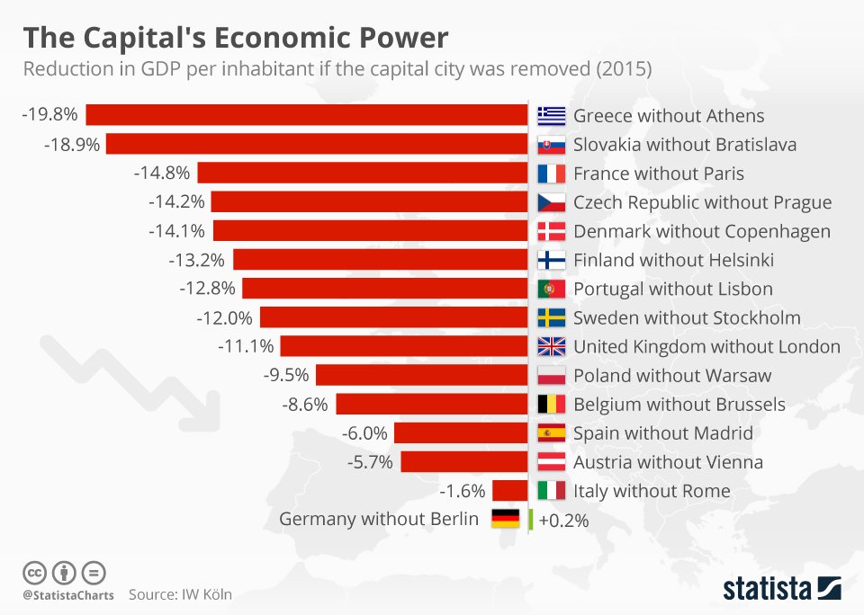
How much does the (financial) capital of a country contribute to its GDP? Which would be India’s city? What would be the reduction in percentage? And these Germans are crazy.(Toc, toc, toc, toc!)
Note how the axis variable that defines the bar locations is a …Qual variable!
There are several Data Visualization packages, even systems, within R.
Base R supports graph making out of the box; (fast, very flexible, but a bit complex)(Update July 2025: There is a new(?) package called
tinyplotsthat creates base R plots with syntax that is much more intuitive. (We will include some here for reference.)The most well known is
ggplothttps://ggplot2-book.org/ which uses Leland Wilkinson’s concept of a “Grammar of Graphics”;ggformulais a wrapper aroundggplotthat makes the syntax a little more concise and intuitive.There is the
latticepackage https://lattice.r-forge.r-project.org/ which uses the “Trellis Graphics” concept framework for data visualization developed by R. A. Becker, W. S. Cleveland, et al.;And the
gridpackage https://bookdown.org/rdpeng/RProgDA/the-grid-package.html that allows extremely fine control ofshapesplotted on the graph.
Each system has its benefits and learning complexities. We will look at plots created using ggformula, and the recently introduced tidyplots package, which allows intuitive creation of publication-ready charts based on the famous and established ggplot framework. We will, where appropriate state ggplot code too for comparison.
A quick reminder on how mosaic and ggformula and ggplot work in a very similar fashion:
mosaic and ggformula command template
Note the standard method for all commands from the mosaic and ggformula packages: goal( y ~ x | z, data = _____)
With mosaic, one can create a statistical correlation test between two variables as: cor_test(y ~ x, data = ______ )
With ggformula, one can create any graph/chart using: gf_***(y ~ x | z, data = _____) In practice, we often use: dataframe %>% gf_***(y ~ x | z) which has cool benefits such as “autocompletion” of variable names, as we shall see. The “***” indicates what kind of graph you desire: histogram, bar, scatter, density; the “___” is the name of your dataset that you want to plot with.
ggplot command template
The ggplot template is used to identify the dataframe, identify the x and y axis, and define visualized layers:
ggplot(data = ---, mapping = aes(x = ---, y = ---)) + geom_----()
Note: —- is meant to imply text you supply. e.g. function names, data frame names, variable names.
It is helpful to see the argument mapping, above. In practice, rather than typing the formal arguments, code is typically shorthanded to this:
dataframe %>% ggplot(aes(xvar, yvar)) + geom_----()
tidyplots command template
tidyplot(data = ---, x = ---, y = ---, color = ---) |> add_***_***()
Bar Charts show counts of observations with respect to a Qualitative variable. For instance, a shop inventory with shirt-sizes. Each bar has a height proportional to the count per shirt-size, in this example.
Although Histograms may look similar to Bar Charts, the two are different. First, histograms show continuous Quant data. By contrast, bar charts show categorical data, such as shirt-sizes, or apples, bananas, carrots, etc. Visually speaking, histograms do not usually show spaces between bars because these are continuous values, while column charts must show spaces to separate each category.
Bar are used to show “counts” and “tallies” with respect to Qual variables: they answer the question How Many?. For instance, in a survey, how many people vs Gender? In a Target Audience survey on Weekly Consumption, how many low, medium, or high expenditure people?
Each Qual variable potentially has many levels as we saw in the Nature of Data. For instance, in the above example on Weekly Expenditure, low, medium and high were levels for the Qual variable Expenditure. Bar charts perform internal counts for each level of the Qual variable under consideration. The Bar Plot is then a set of disjoint bars representing these counts; see the icon above, and then that for histograms!! The X-axis is the set of levels in the Qual variable, and the Y-axis represents the counts for each level.
We will first look at at a dataset that speaks about taxi rides in Chicago in the year 2022. This is available on Vincent Arel-Bundock’s superb repository of datasets.Let us read into R directly from the website.
taxi <- read_csv("https://vincentarelbundock.github.io/Rdatasets/csv/modeldata/taxi.csv")The data has automatically been read into the webr session, so you can continue on to the next code chunk!
Loading webR...
As per our Workflow, we will look at the data using all the three methods we have seen.
dplyr::glimpse(taxi)Rows: 10,000
Columns: 8
$ rownames <dbl> 1, 2, 3, 4, 5, 6, 7, 8, 9, 10, 11, 12, 13, 14, 15, 16, 17, 18…
$ tip <chr> "yes", "yes", "yes", "yes", "yes", "yes", "yes", "yes", "yes"…
$ distance <dbl> 17.19, 0.88, 18.11, 20.70, 12.23, 0.94, 17.47, 17.67, 1.85, 1…
$ company <chr> "Chicago Independents", "City Service", "other", "Chicago Ind…
$ local <chr> "no", "yes", "no", "no", "no", "yes", "no", "no", "no", "no",…
$ dow <chr> "Thu", "Thu", "Mon", "Mon", "Sun", "Sat", "Fri", "Sun", "Fri"…
$ month <chr> "Feb", "Mar", "Feb", "Apr", "Mar", "Apr", "Mar", "Jan", "Apr"…
$ hour <dbl> 16, 8, 18, 8, 21, 23, 12, 6, 12, 14, 18, 11, 12, 19, 17, 13, …skimr::skim(taxi)| Name | taxi |
| Number of rows | 10000 |
| Number of columns | 8 |
| _______________________ | |
| Column type frequency: | |
| character | 5 |
| numeric | 3 |
| ________________________ | |
| Group variables | None |
Variable type: character
| skim_variable | n_missing | complete_rate | min | max | empty | n_unique | whitespace |
|---|---|---|---|---|---|---|---|
| tip | 0 | 1 | 2 | 3 | 0 | 2 | 0 |
| company | 0 | 1 | 5 | 28 | 0 | 7 | 0 |
| local | 0 | 1 | 2 | 3 | 0 | 2 | 0 |
| dow | 0 | 1 | 3 | 3 | 0 | 7 | 0 |
| month | 0 | 1 | 3 | 3 | 0 | 4 | 0 |
Variable type: numeric
| skim_variable | n_missing | complete_rate | mean | sd | p0 | p25 | p50 | p75 | p100 | hist |
|---|---|---|---|---|---|---|---|---|---|---|
| rownames | 0 | 1 | 5000.50 | 2886.90 | 1 | 2500.75 | 5000.50 | 7500.25 | 10000.0 | ▇▇▇▇▇ |
| distance | 0 | 1 | 6.22 | 7.38 | 0 | 0.94 | 1.78 | 15.56 | 42.3 | ▇▁▂▁▁ |
| hour | 0 | 1 | 14.18 | 4.36 | 0 | 11.00 | 15.00 | 18.00 | 23.0 | ▁▃▅▇▃ |
mosaic::inspect(taxi)
categorical variables:
name class levels n missing
1 tip character 2 10000 0
2 company character 7 10000 0
3 local character 2 10000 0
4 dow character 7 10000 0
5 month character 4 10000 0
distribution
1 yes (92.1%), no (7.9%)
2 other (27.1%) ...
3 no (81.2%), yes (18.8%)
4 Thu (19.6%), Wed (17.5%), Tue (16.3%) ...
5 Apr (31.8%), Mar (31.4%), Feb (20.4%) ...
quantitative variables:
name class min Q1 median Q3 max mean
1 rownames numeric 1 2500.75 5000.50 7500.2500 10000.0 5000.500000
2 distance numeric 0 0.94 1.78 15.5625 42.3 6.224144
3 hour numeric 0 11.00 15.00 18.0000 23.0 14.177300
sd n missing
1 2886.895680 10000 0
2 7.381397 10000 0
3 4.359904 10000 0
-
distance: Continuous Quant variable, the distance of the trip in miles.
-
tip: Yes/No type Qual variable, whether a tip was given or not. -
company: 7 levels, the cab company that was used for the ride. -
local: 2 levels, whether the trip was local or not. -
hour: 24 levels, the hour of the day when the trip started. -
dow: 7 levels, the day of the week. -
month: 12 levels, the month of the year.
taxi dataset
- This is a large dataset (10K rows), 8 columns/variables.
- There are several Qualitative variables:
tip(2),company(7) andlocal(2),dow(7), andmonth(12). These have levels as shown in the parenthesis. - Note that
hourdespite being a discrete/numerical variable, it can be treated as a Categorical variable too. -
distanceis Quantitative. - There are no missing values for any variable, all are complete with 10K entries.
We will convert the tip, company, dow, local, hour, and month variables into factors beforehand.
## Convert `dow`, `local`, `month`, and `hour` into ordered factors
taxi_modified <- taxi %>%
mutate(
##
tip = factor(tip,
levels = c("yes", "no"),
labels = c("yes", "no"),
ordered = TRUE
),
##
company = factor(company), # Any order is OK.
##
dow = factor(dow,
levels = c("Mon", "Tue", "Wed", "Thu", "Fri", "Sat", "Sun"),
labels = c("Mon", "Tue", "Wed", "Thu", "Fri", "Sat", "Sun"),
ordered = TRUE
),
##
local = factor(local,
levels = c("yes", "no"),
labels = c("yes", "no"),
ordered = TRUE
),
##
month = factor(month,
levels = c("Jan", "Feb", "Mar", "Apr"),
labels = c("Jan", "Feb", "Mar", "Apr"),
ordered = TRUE
),
##
hour = factor(hour,
levels = c(0:23), labels = c(0:23),
ordered = TRUE
)
)
taxi_modified %>% glimpse()Rows: 10,000
Columns: 8
$ rownames <dbl> 1, 2, 3, 4, 5, 6, 7, 8, 9, 10, 11, 12, 13, 14, 15, 16, 17, 18…
$ tip <ord> yes, yes, yes, yes, yes, yes, yes, yes, yes, yes, yes, yes, y…
$ distance <dbl> 17.19, 0.88, 18.11, 20.70, 12.23, 0.94, 17.47, 17.67, 1.85, 1…
$ company <fct> Chicago Independents, City Service, other, Chicago Independen…
$ local <ord> no, yes, no, no, no, yes, no, no, no, no, no, no, no, yes, no…
$ dow <ord> Thu, Thu, Mon, Mon, Sun, Sat, Fri, Sun, Fri, Tue, Tue, Sun, W…
$ month <ord> Feb, Mar, Feb, Apr, Mar, Apr, Mar, Jan, Apr, Mar, Mar, Apr, A…
$ hour <ord> 16, 8, 18, 8, 21, 23, 12, 6, 12, 14, 18, 11, 12, 19, 17, 13, …Loading webR...
The target variable for an experiment that resulted in this data might be the tip variable, since that looks like a response, or an outcome. It is a binary i.e. Yes/No type Qual variable.
We will use the tip variable to ask questions about the data, and then plot the answers to these questions.
- Do more people
tipthan not? - Does a
tipdepend upon whether the trip islocalor not? - Do some cab
company-ies get more tips than others? - And does a
tipdepend upon thedistance,hourof day, anddowandmonth?
Try and think of more Questions!
Let’s plot some bar graphs: recall that for bar charts, we need to choose Qual variables to count with! In each case, we will state a Hypothesis/Question and try to answer it with a chart.
tip than not?
tip than not?

Show the Code
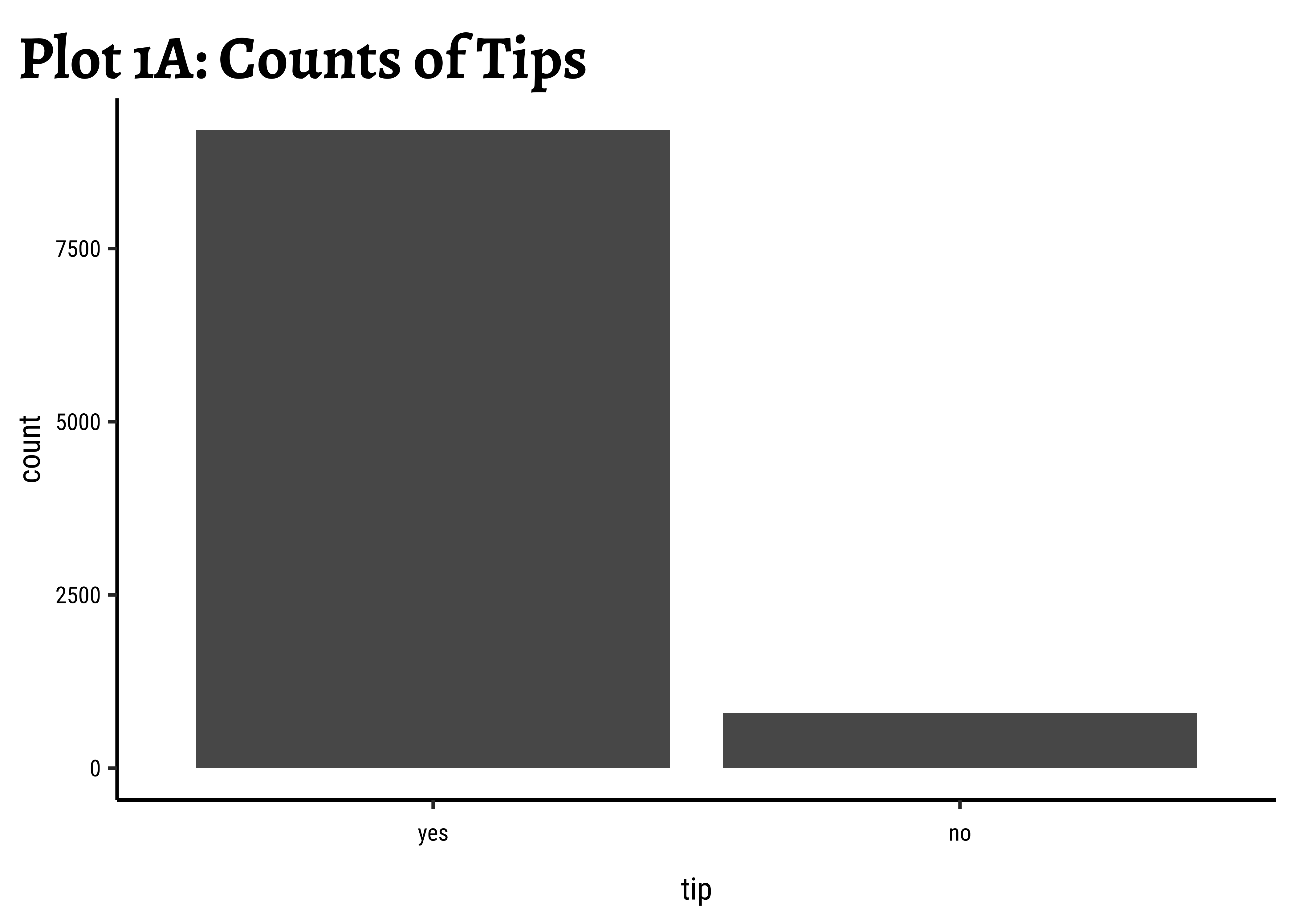
tidyplot(x = tip, data = taxi_modified) %>%
add_count_bar() %>%
add_title("Plot 1A: Counts of Tips") %>%
adjust_size(height = 50, width = 85, unit = "mm") %>%
adjust_colors(colors_discrete_friendly)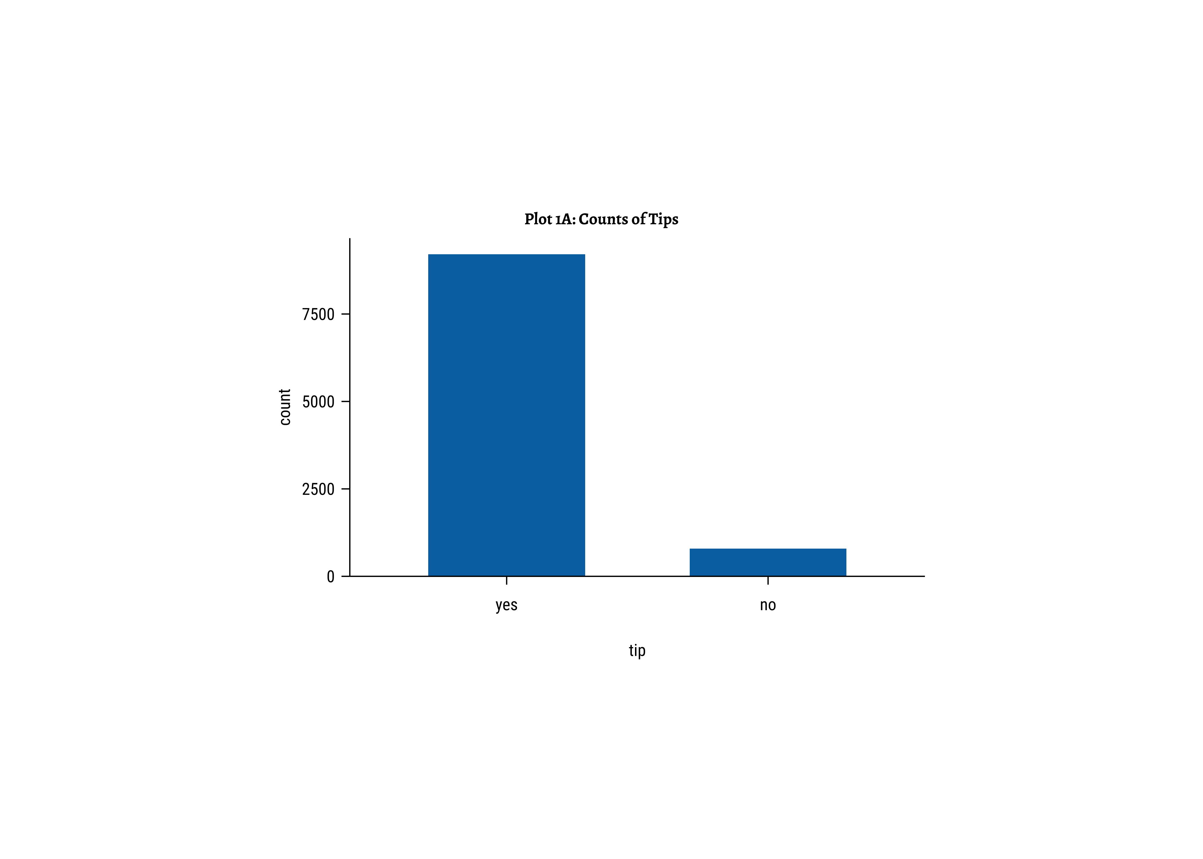
Show the Code
tinyplot(~tip,
data = taxi_modified,
type = "barplot",
main = "Plot 1A: Counts of Tips"
)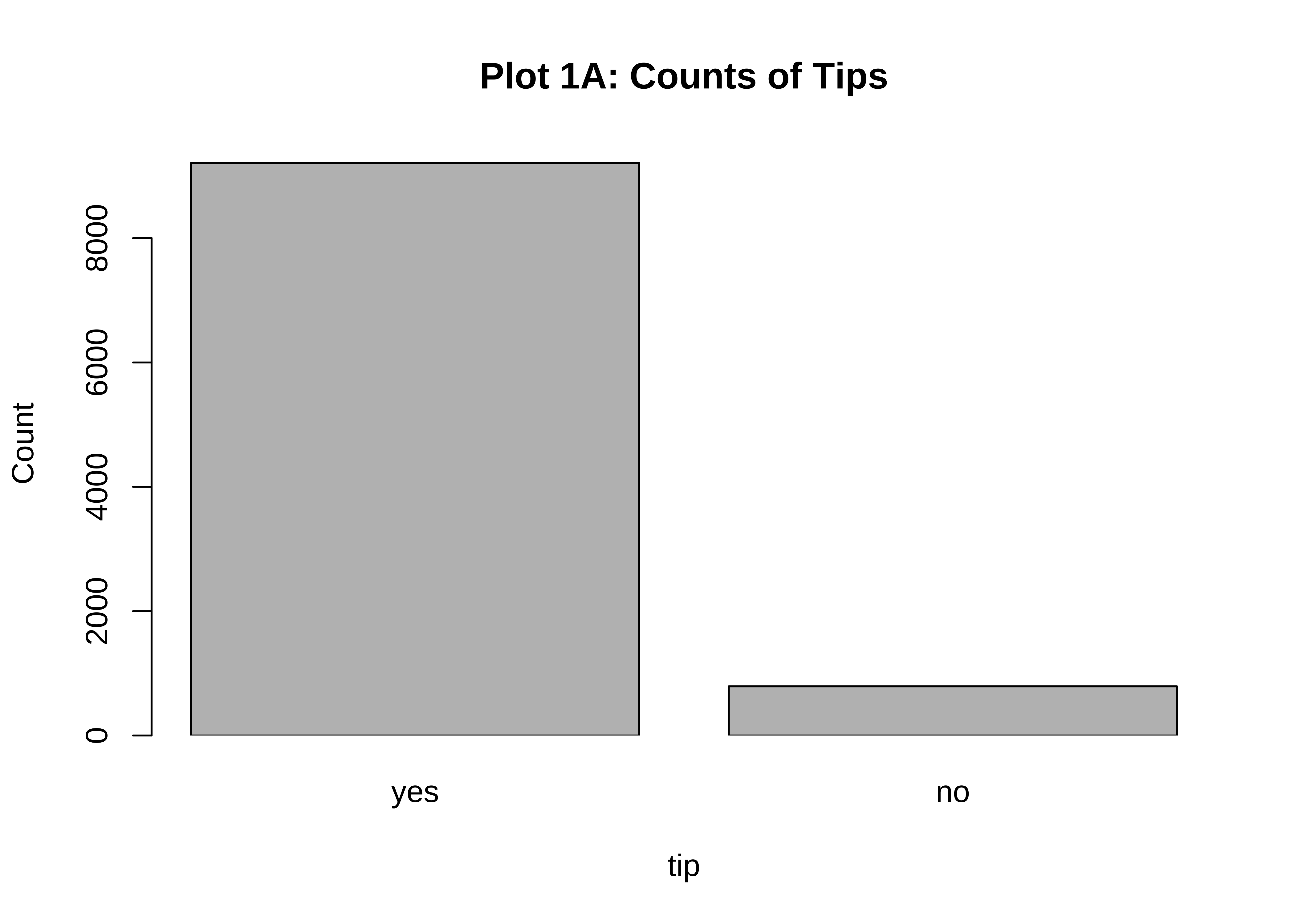
Business Insights-1
- Far more people do
tipthan not. Which is nice. - (Future) The counts of
tipare very imbalanced and if we are to setup a model for that (logistic regression) we would need to very carefully subset the data fortrainingandtestingour model.
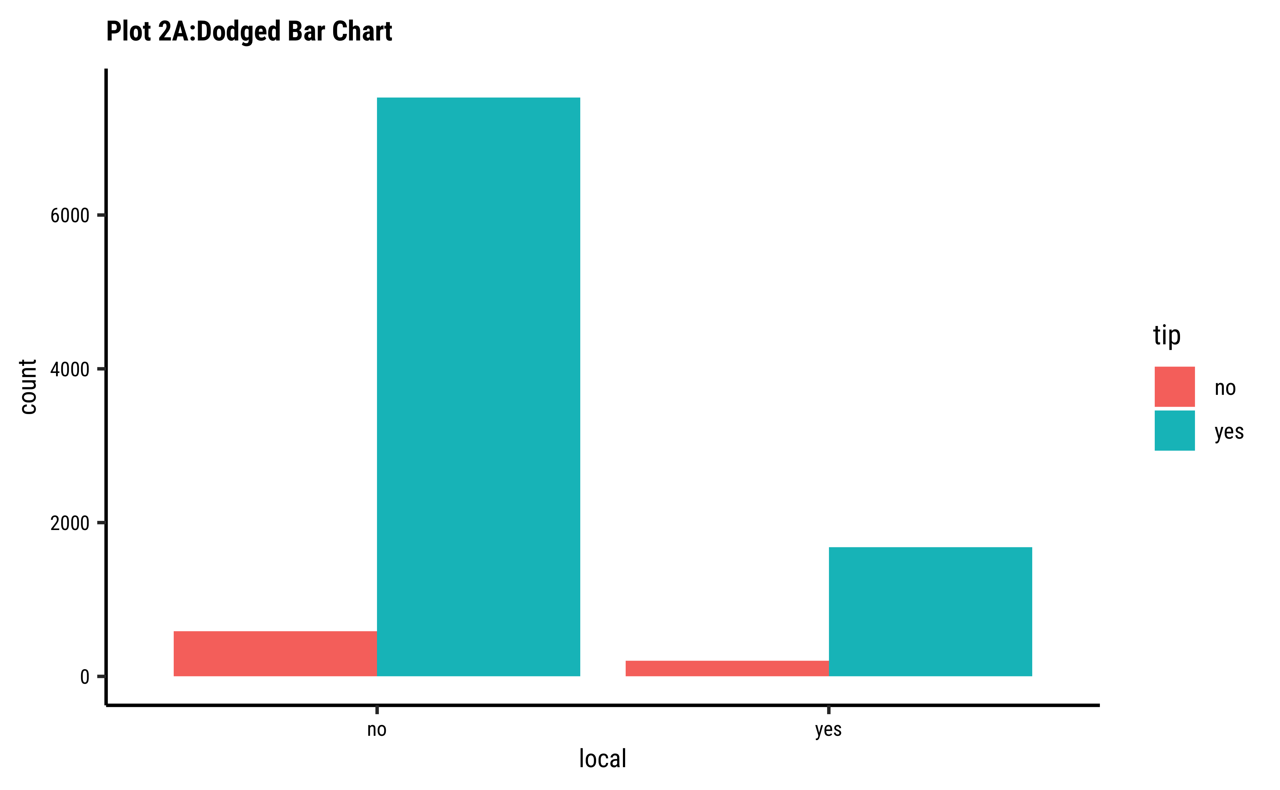
tip depend upon whether the trip is local or not?
tip depend upon whether the trip is local or not?


theme_set(new = theme_custom())
## Showing "per capita" percentages
## Better labelling of Y-axis
taxi_modified %>%
gf_props(~local,
fill = ~tip,
position = "fill"
) %>%
gf_labs(
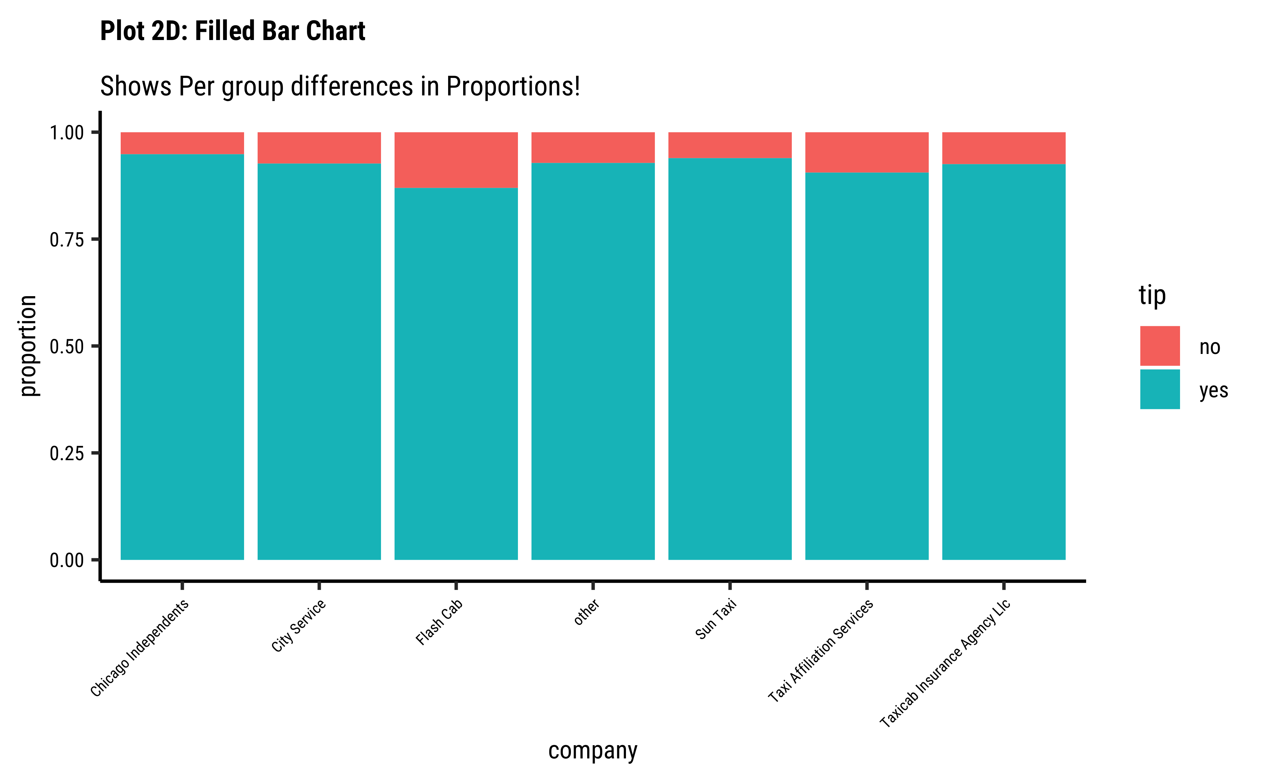
title = "Plot 2D: Filled Bar Chart",
subtitle = "Shows Per group differences in Proportions!"
) %>%
gf_refine(scale_fill_brewer(palette = "Set1"))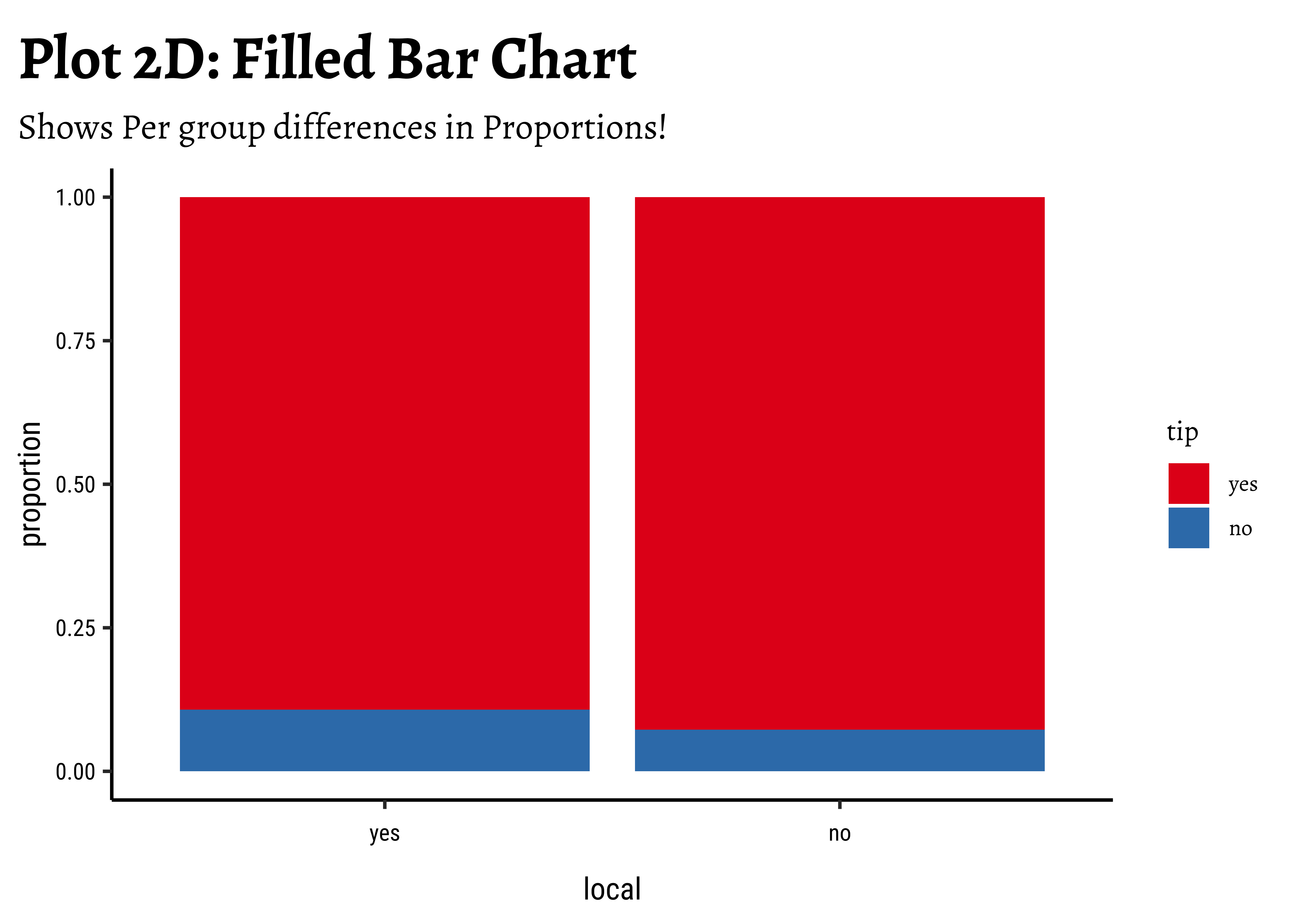
theme_set(new = theme_custom())
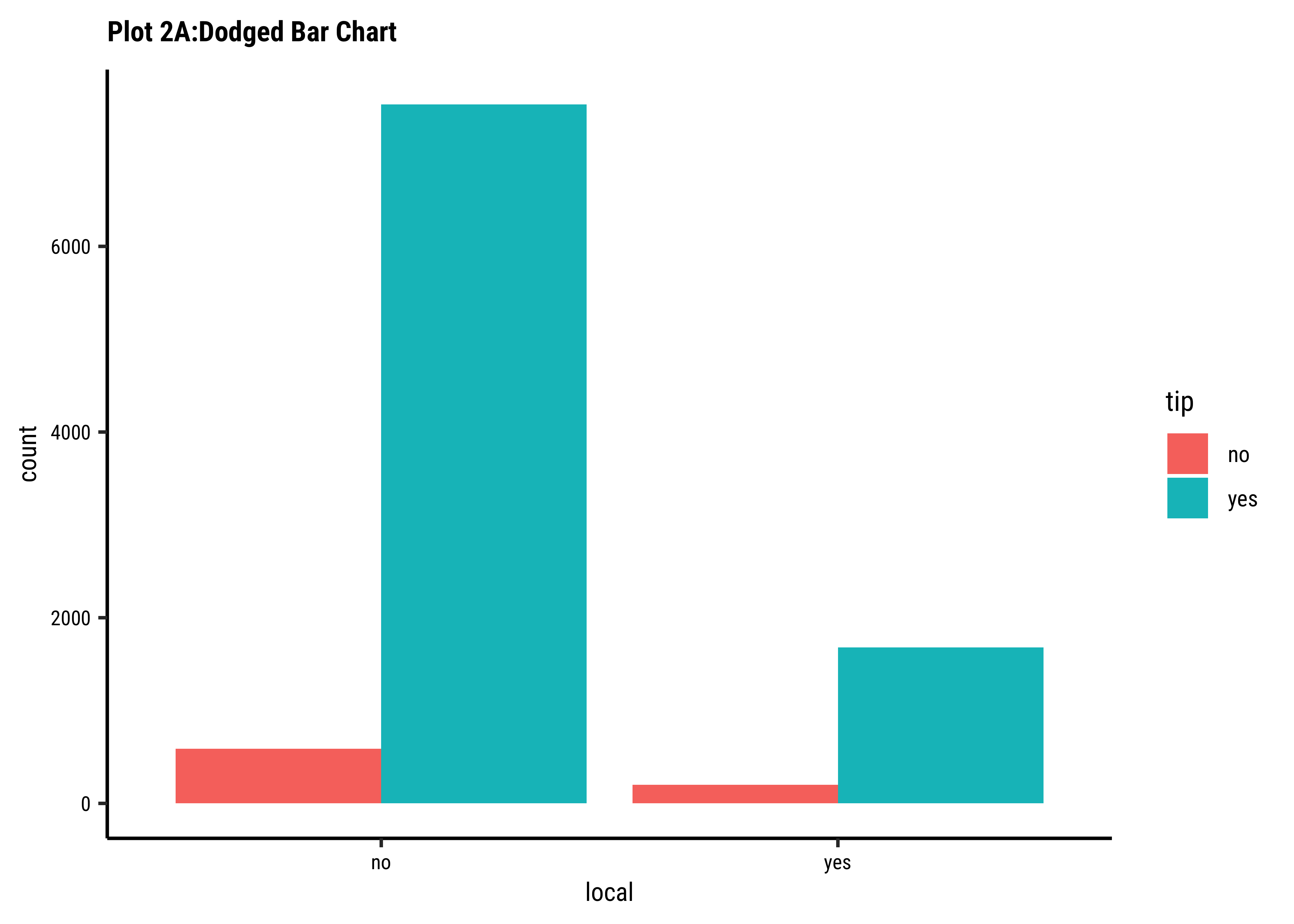
taxi_modified %>%
ggplot() +
geom_bar(aes(x = local, fill = tip), position = "dodge") +
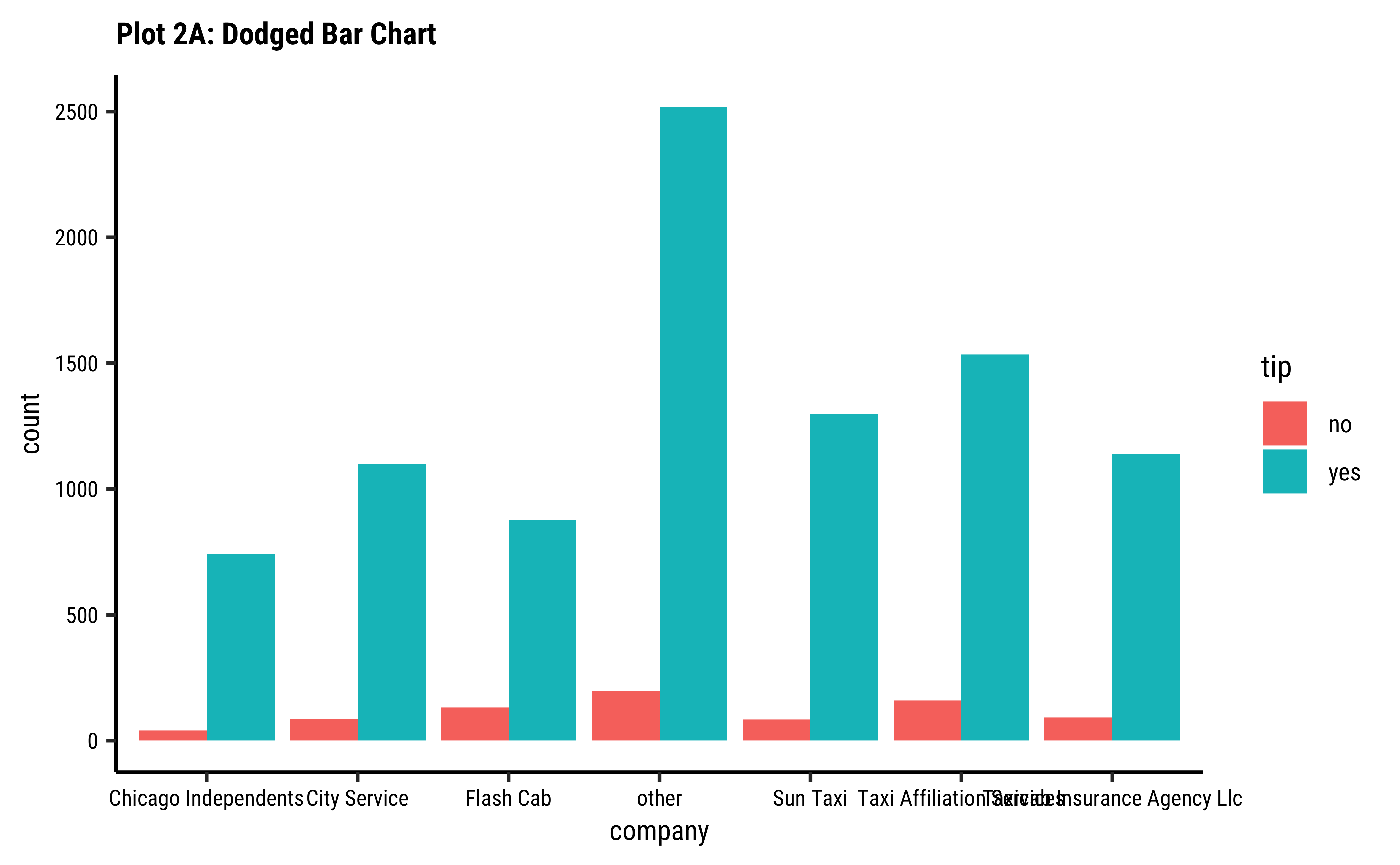
labs(title = "Plot 2A:Dodged Bar Chart") +
scale_fill_brewer(palette = "Set1")
##
taxi_modified %>%
ggplot() +
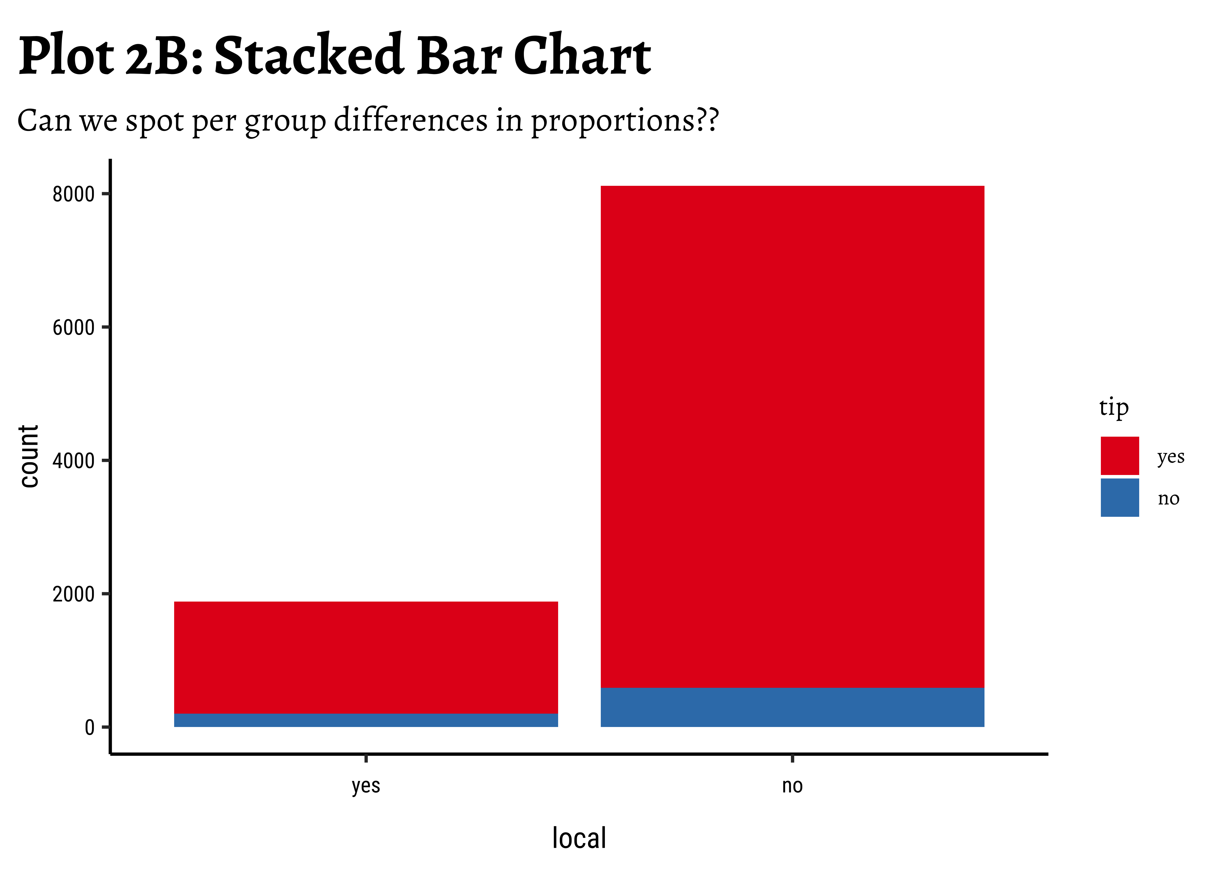
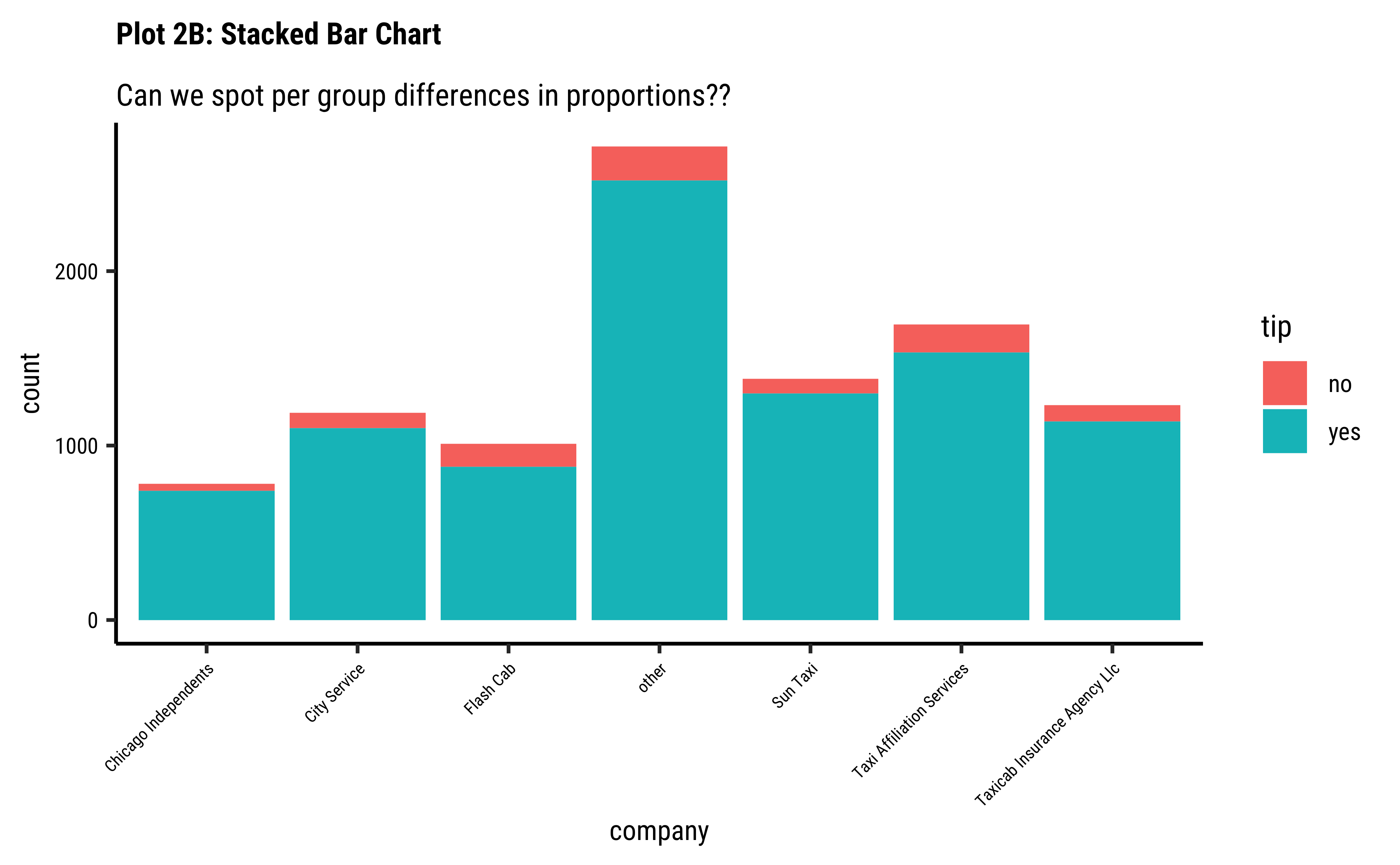
geom_bar(aes(x = local, fill = tip), position = "stack") +
labs(
title = "Plot 2B: Stacked Bar Chart",
subtitle = "Can we spot per group differences in proportions??"
) +
scale_fill_brewer(palette = "Set1")
## Showing "per capita" percentages
taxi_modified %>%
ggplot() +
geom_bar(aes(x = local, fill = tip), position = "fill") +
labs(title = "Plot 2C: Filled Bar Chart", subtitle = "Shows Per group differences in Proportions!") +
scale_fill_brewer(palette = "Set1")
## Showing "per capita" percentages
## Better labelling of Y-axis
taxi_modified %>%
ggplot() +
geom_bar(aes(x = local, fill = tip), position = "fill") +
labs(
title = "Plot 2D: Filled Bar Chart",
subtitle = "Shows Per group differences in Proportions!",
y = "Proportion"
) +
scale_fill_brewer(palette = "Set1")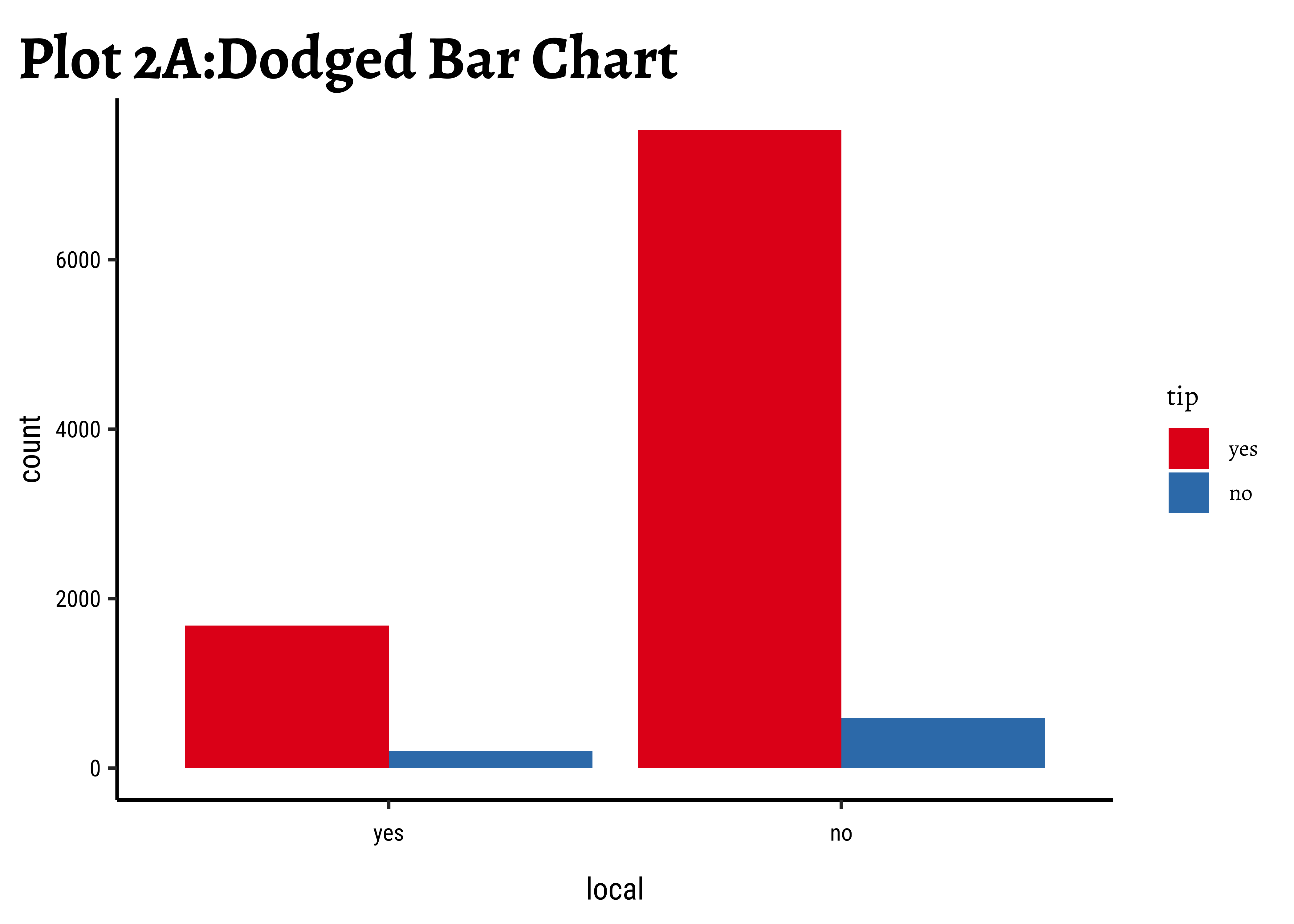


tidyplots::tidyplot(local,
colour = tip,
data = taxi_modified
) %>%
add_count_bar() %>%
add_title("Plot 2A: Dodged Bar Chart") %>%
adjust_size(height = 50, width = 80, unit = "mm") %>%
adjust_colors(colors_discrete_friendly)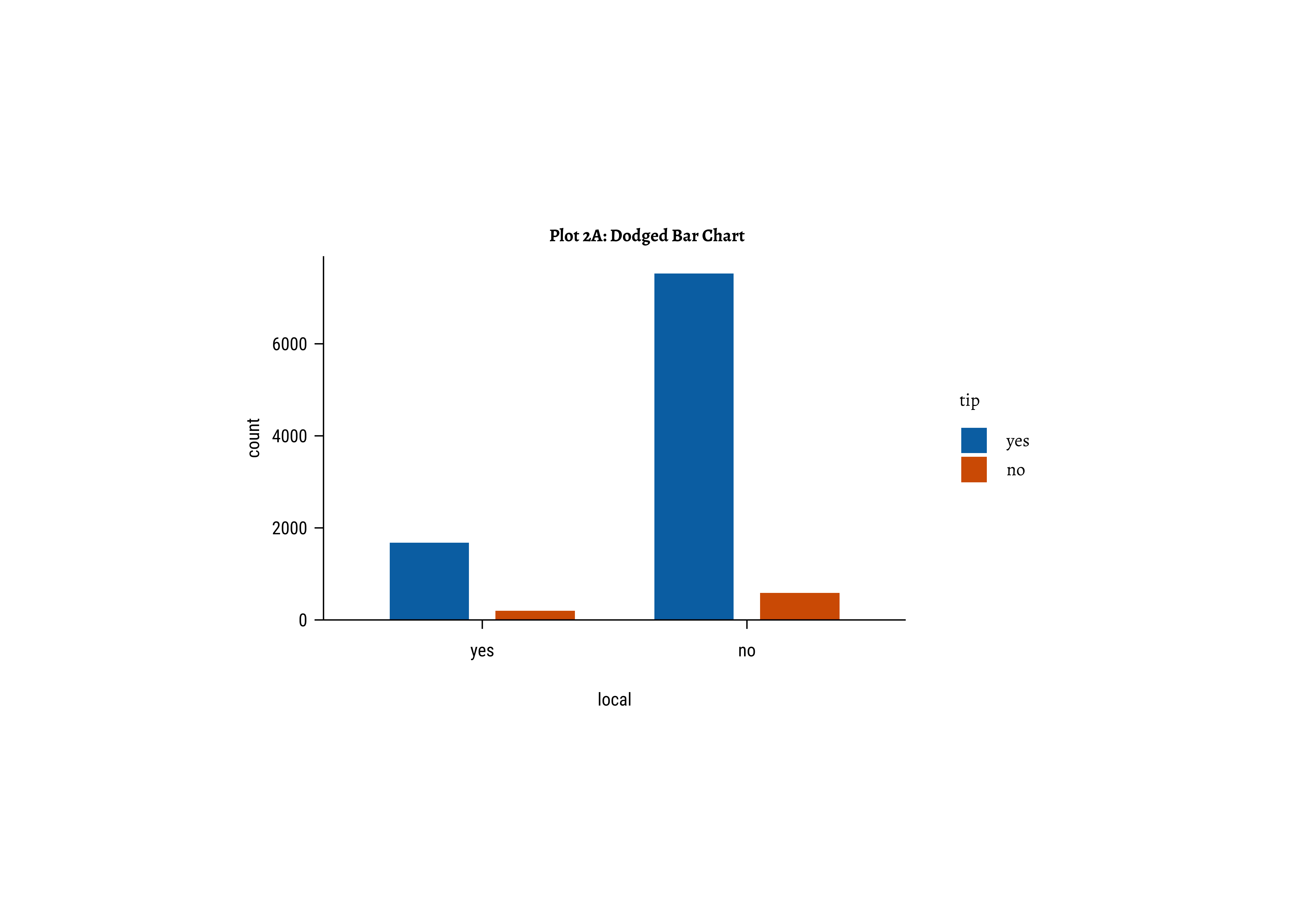
tidyplots::tidyplot(local, colour = tip, data = taxi_modified) %>%
add_barstack_absolute() %>%
add_title("Plot 2B: Stacked Bar Chart") %>%
adjust_size(height = 50, width = 80, unit = "mm") %>%
adjust_colors(colors_discrete_friendly)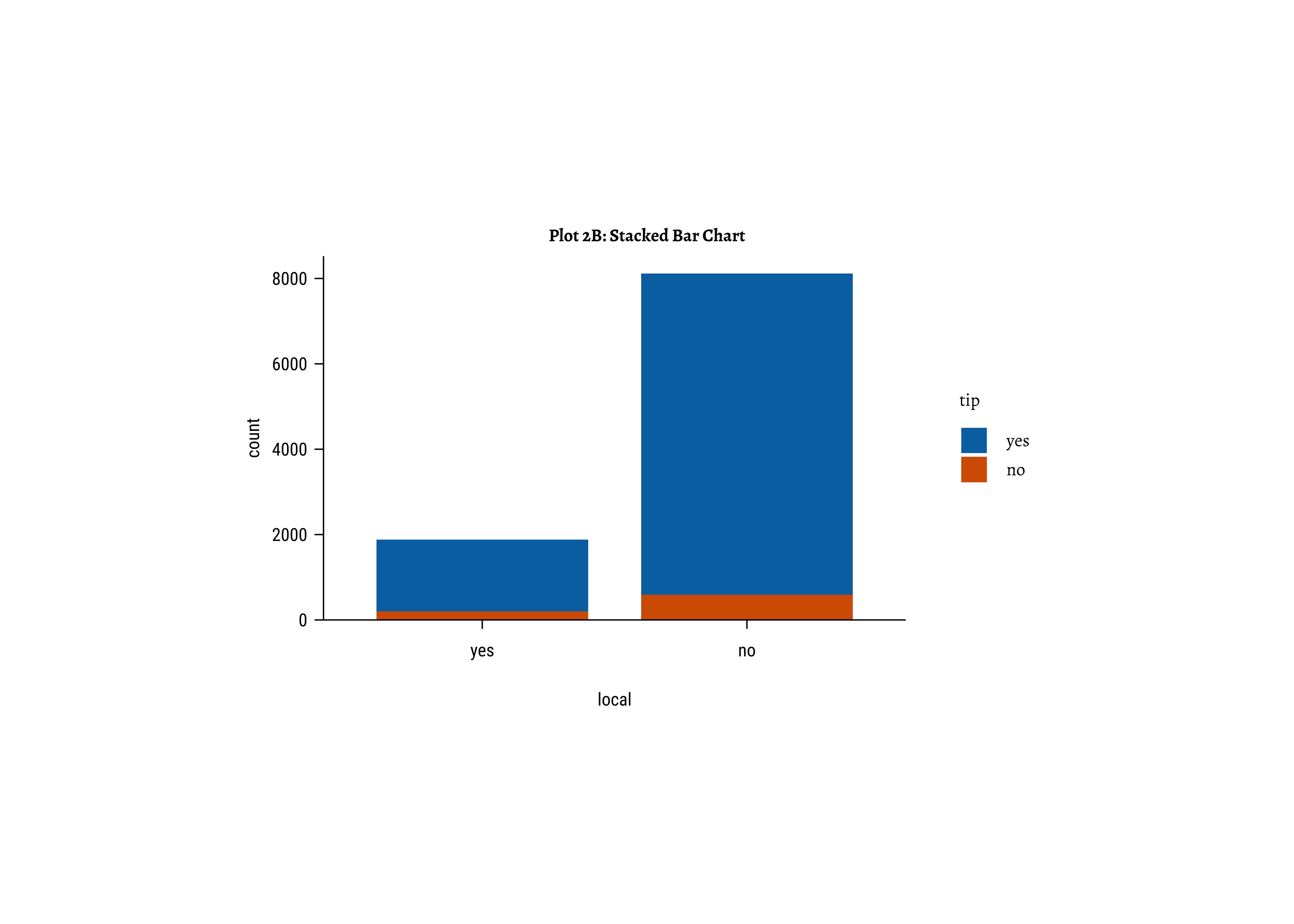
tidyplots::tidyplot(local,
colour = tip,
data = taxi_modified
) %>%
add_barstack_relative() %>%
add_title("Plot 2C: Dodged Bar Chart") %>%
adjust_size(height = 50, width = 80, unit = "mm") %>%
adjust_colors(colors_discrete_friendly)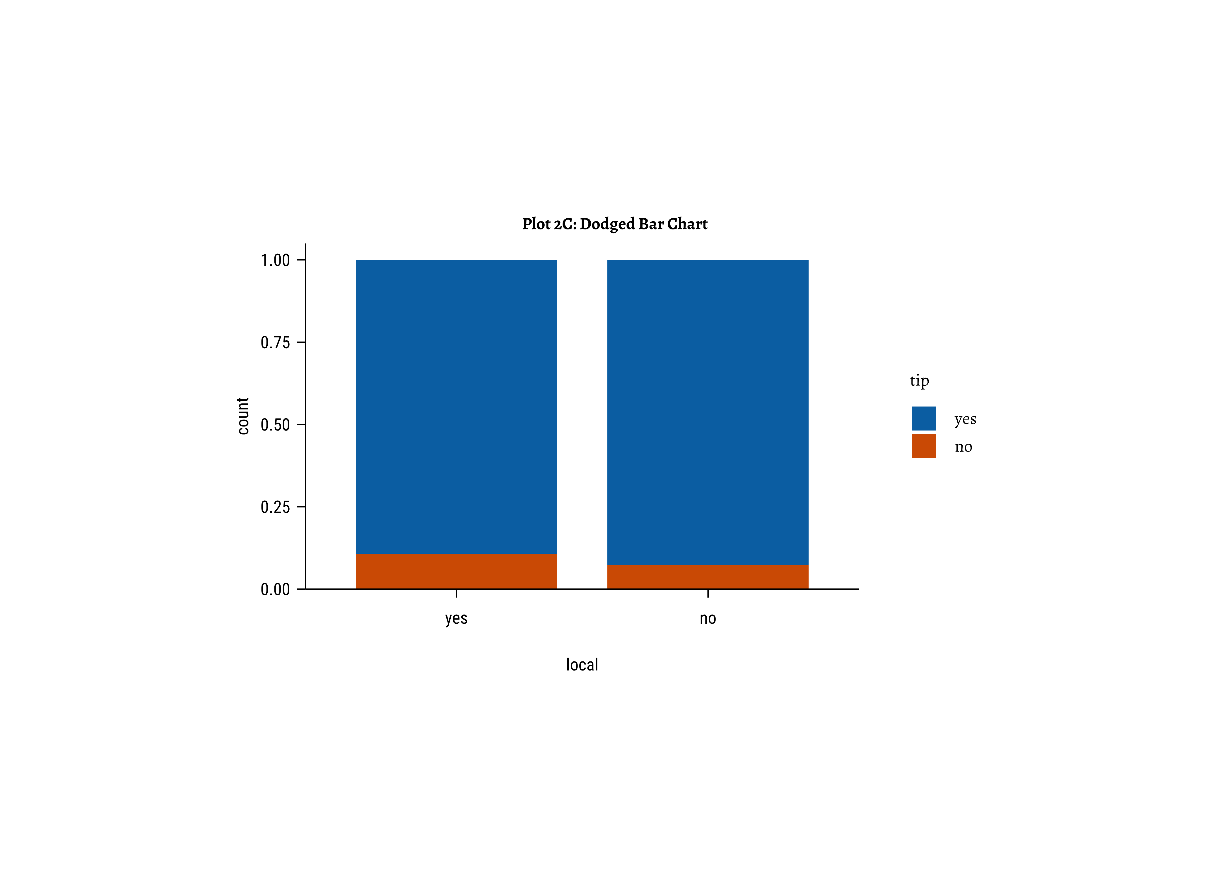
tinyplot(~ local | tip,
data = taxi_modified,
type = "barplot", palette = "tableau",
beside = TRUE, # for placing bars beside one another
main = "Plot 2A: Dodged Bar Chart",
legend = "right!"
) # Outside, to the right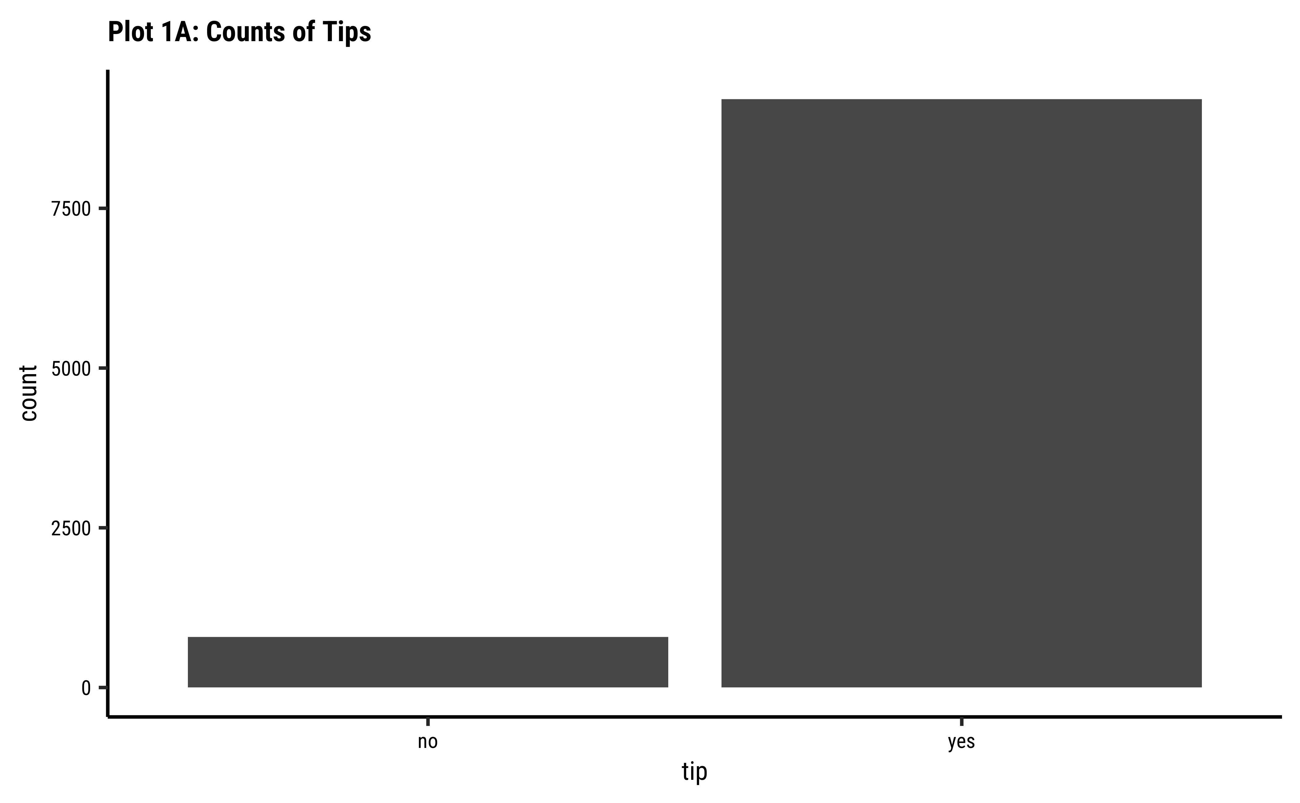

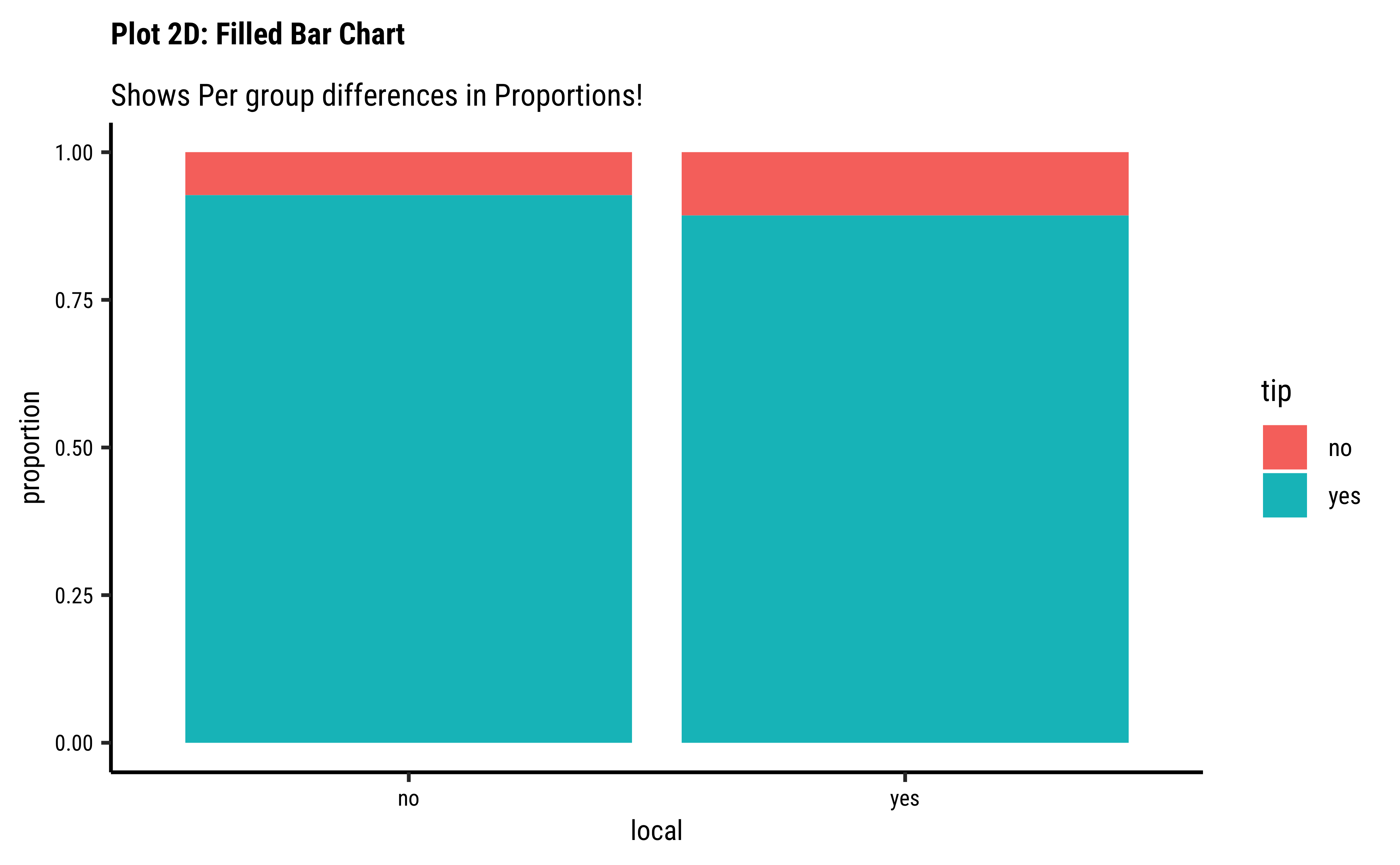
Business Insights-2
- Counting the frequency of
tipbylocalgives us grouped counts, but we cannot tell the percentage per group (local or not) of those who tip and those who do not. - We need per-group percentages because the number of
localtrips are not balanced - Hence with
tidyplots, we find thatadd_barstack_relativegives the clearest visual indication of a difference in proportion. - Likewise with
ggformula, we tried bar charts withposition = stack, but finally it is theposition = fillthat works best. - We see that the percentage of tippers is somewhat higher with people who make non-local trips. Not surprising.
company-ies get more tips than others?
company-ies get more tips than others?
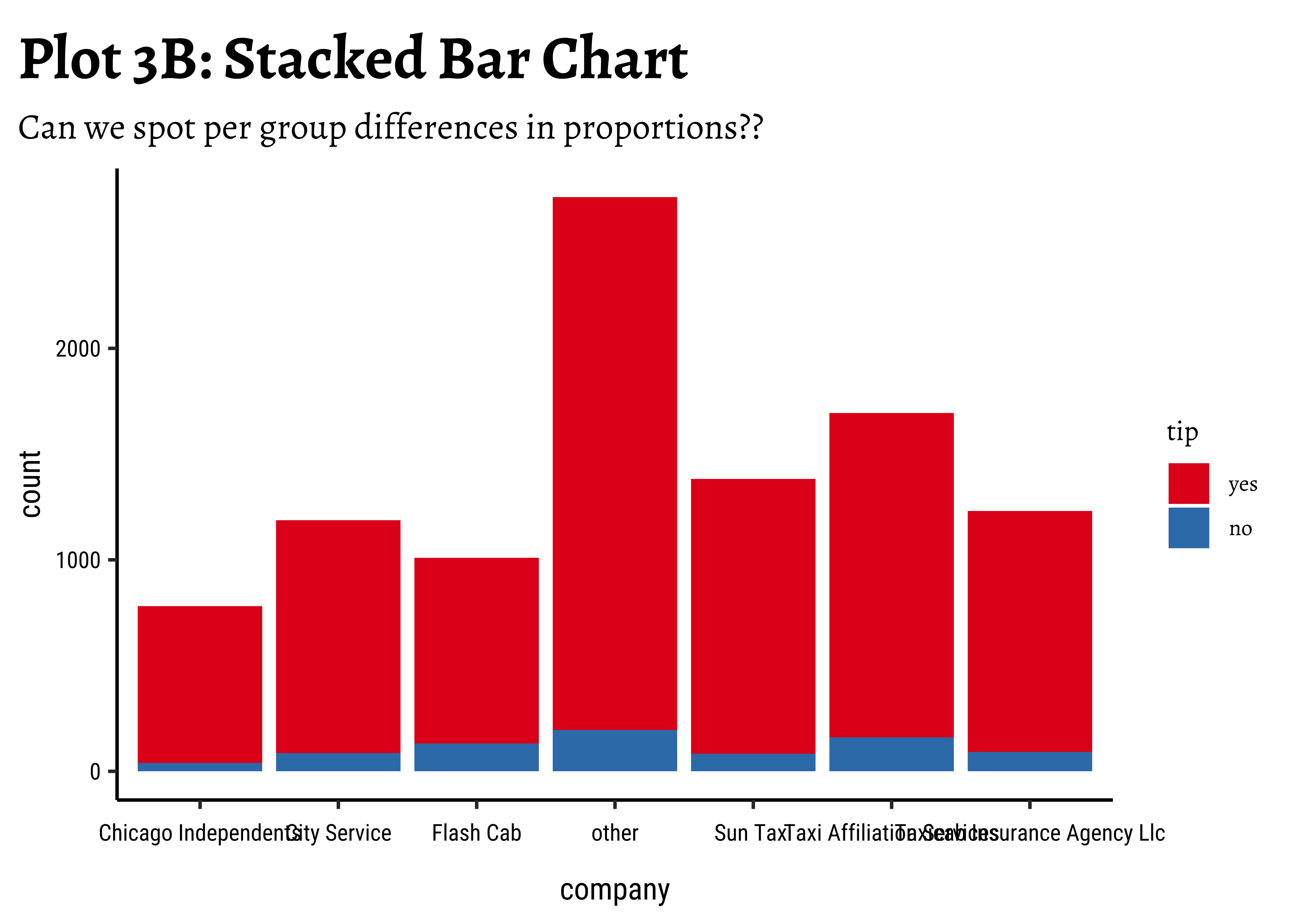
theme_set(new = theme_custom())
taxi_modified %>%
gf_bar(~company, fill = ~tip, position = "stack") %>%
gf_labs(
title = "Plot 3B: Stacked Bar Chart",
subtitle = "Can we spot per group differences in proportions??"
) %>%
gf_theme(theme(axis.text.x = element_text(size = 6, angle = 45, hjust = 1))) %>%
gf_refine(scale_fill_brewer(palette = "Set1"))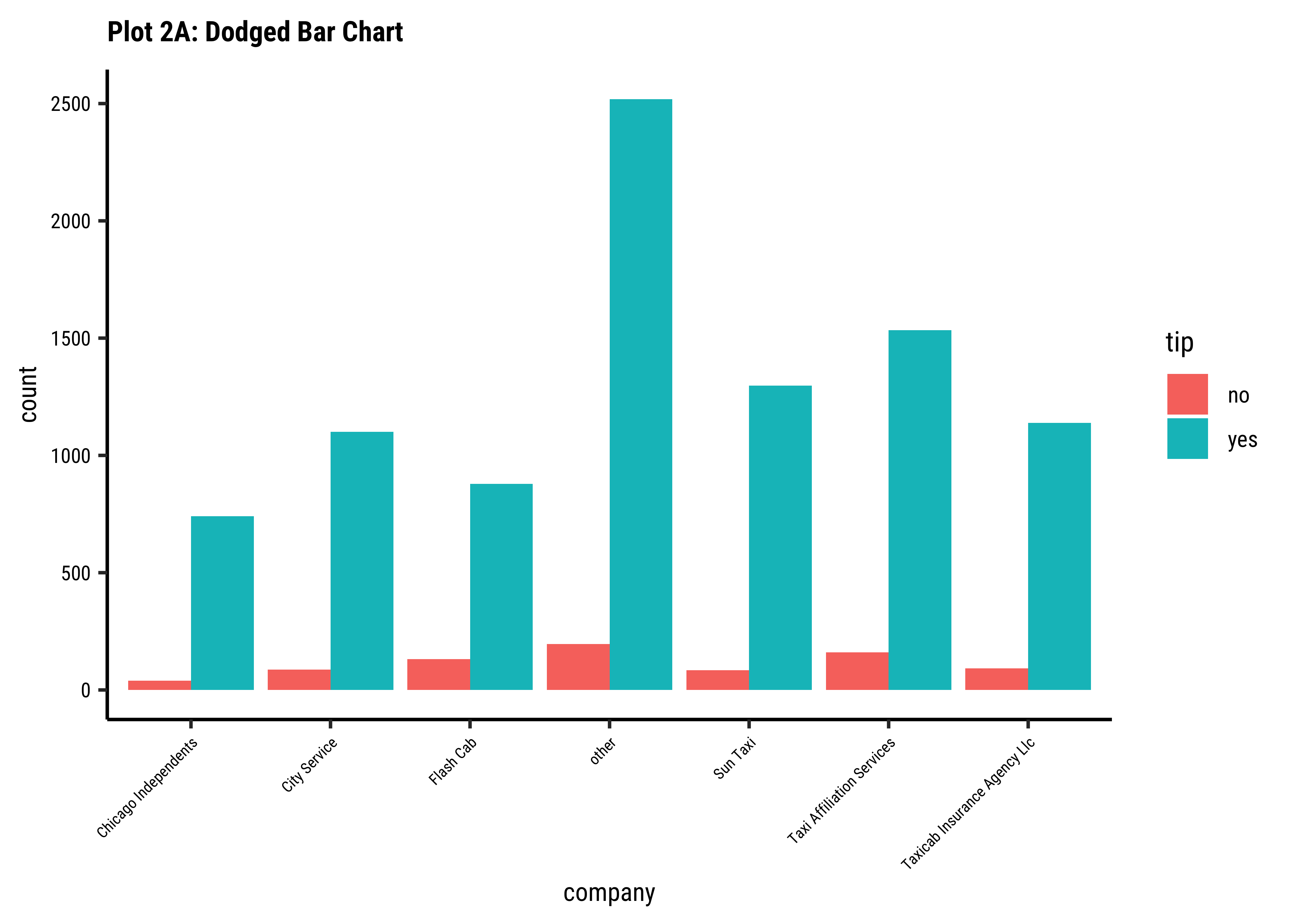
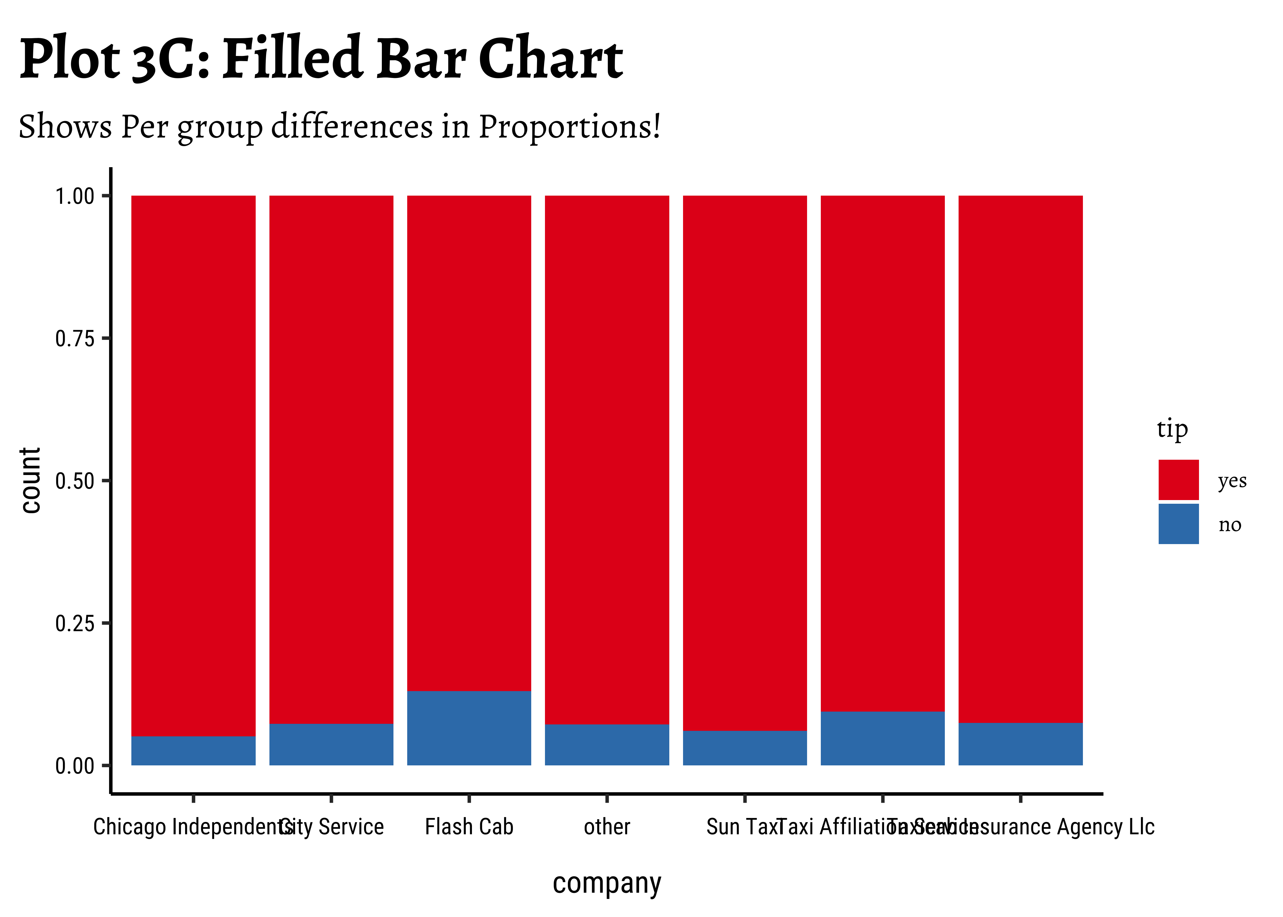
theme_set(new = theme_custom())
## Showing "per capita" percentages
taxi_modified %>%
gf_percents(~company, fill = ~tip, position = "fill") %>%
gf_labs(
title = "Plot 3C: Filled Bar Chart",
subtitle = "Shows Per group differences in Proportions!"
) %>%
gf_theme(theme(axis.text.x = element_text(size = 6, angle = 45, hjust = 1))) %>%
gf_refine(scale_fill_brewer(palette = "Set1"))
theme_set(new = theme_custom())
## Showing "per capita" percentages
## Better labelling of Y-axis
taxi_modified %>%
gf_props(~company, fill = ~tip, position = "fill") %>%
gf_labs(
title = "Plot 3D: Filled Bar Chart",
subtitle = "Shows Per group differences in Proportions!"
) %>%
gf_theme(theme(axis.text.x = element_text(size = 6, angle = 45, hjust = 1))) %>%
gf_refine(scale_fill_brewer(palette = "Set1"))
theme_set(new = theme_custom())
taxi_modified %>%
ggplot() +
geom_bar(aes(x = company, fill = tip), position = "dodge") +
labs(title = "Plot 3A: Dodged Bar Chart") +
theme(theme(axis.text.x = element_text(size = 6, angle = 45, hjust = 1))) +
scale_fill_brewer(palette = "Set1")
##
taxi_modified %>%
ggplot() +
geom_bar(aes(x = company, fill = tip), position = "stack") +
labs(
title = "Plot 3B: Stacked Bar Chart",
subtitle = "Can we spot per group differences in proportions??"
) +
theme(theme(axis.text.x = element_text(size = 6, angle = 45, hjust = 1))) +
scale_fill_brewer(palette = "Set1")
## Showing "per capita" percentages
taxi_modified %>%
ggplot() +
geom_bar(aes(x = company, fill = tip), position = "fill") +
labs(
title = "Plot 3C: Filled Bar Chart",
subtitle = "Shows Per group differences in Proportions!"
) +
theme(theme(axis.text.x = element_text(size = 6, angle = 45, hjust = 1))) +
scale_fill_brewer(palette = "Set1")
## Showing "per capita" percentages
## Better labelling of Y-axis
taxi_modified %>%
ggplot() +
geom_bar(aes(x = company, fill = tip), position = "fill") +
labs(
title = "Plot 3D: Filled Bar Chart",
subtitle = "Shows Per group differences in Proportions!",
y = "Proportions"
) +
theme(theme(axis.text.x = element_text(size = 6, angle = 45, hjust = 1))) +
scale_fill_brewer(palette = "Set1")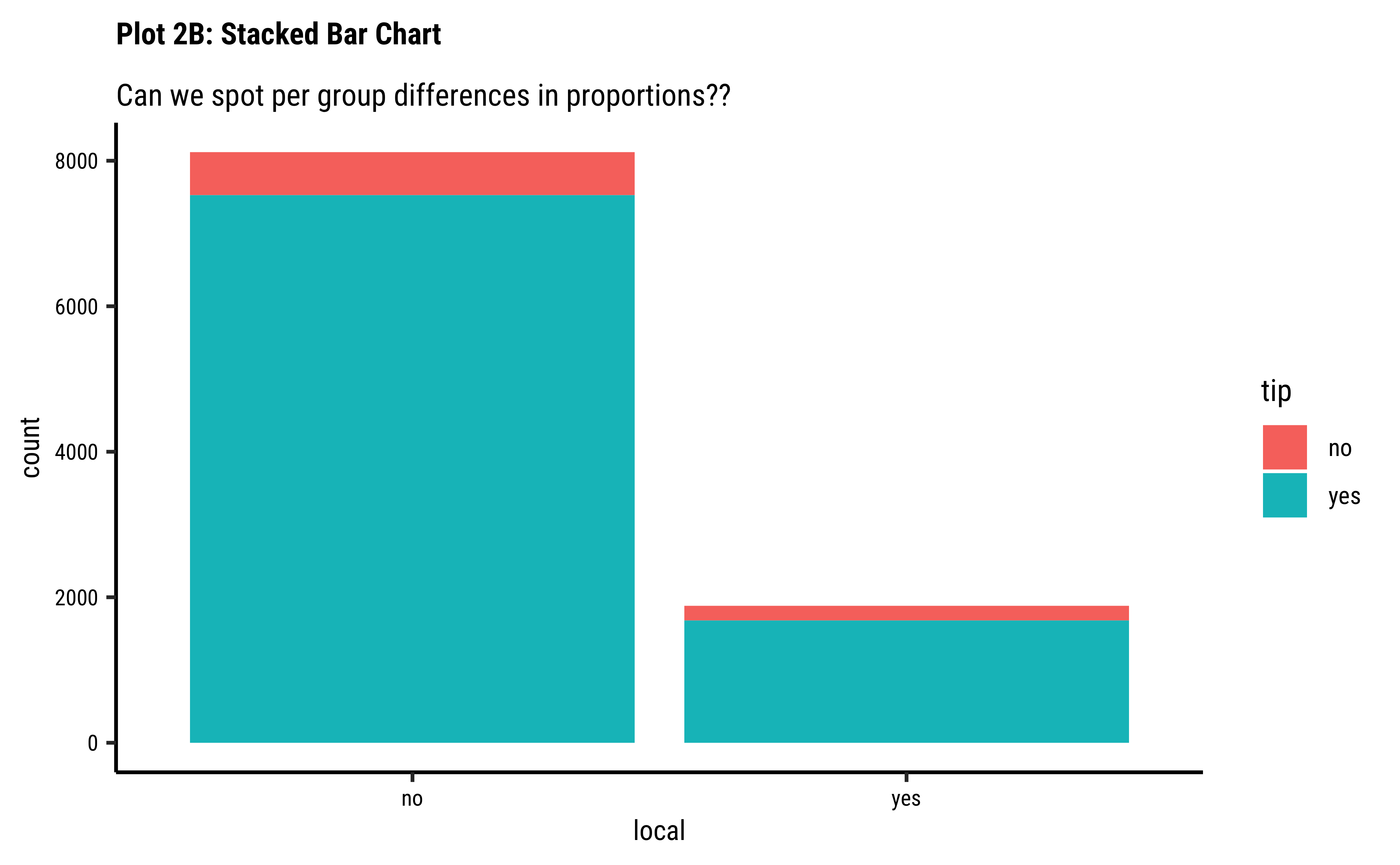

tidyplots::tidyplot(company,
colour = tip,
data = taxi_modified
) %>%
add_count_bar() %>%
add_title("Plot 3A: Dodged Bar Chart") %>%
adjust_size(height = 50, width = 80, unit = "mm") %>%
adjust_x_axis(rotate_labels = 45)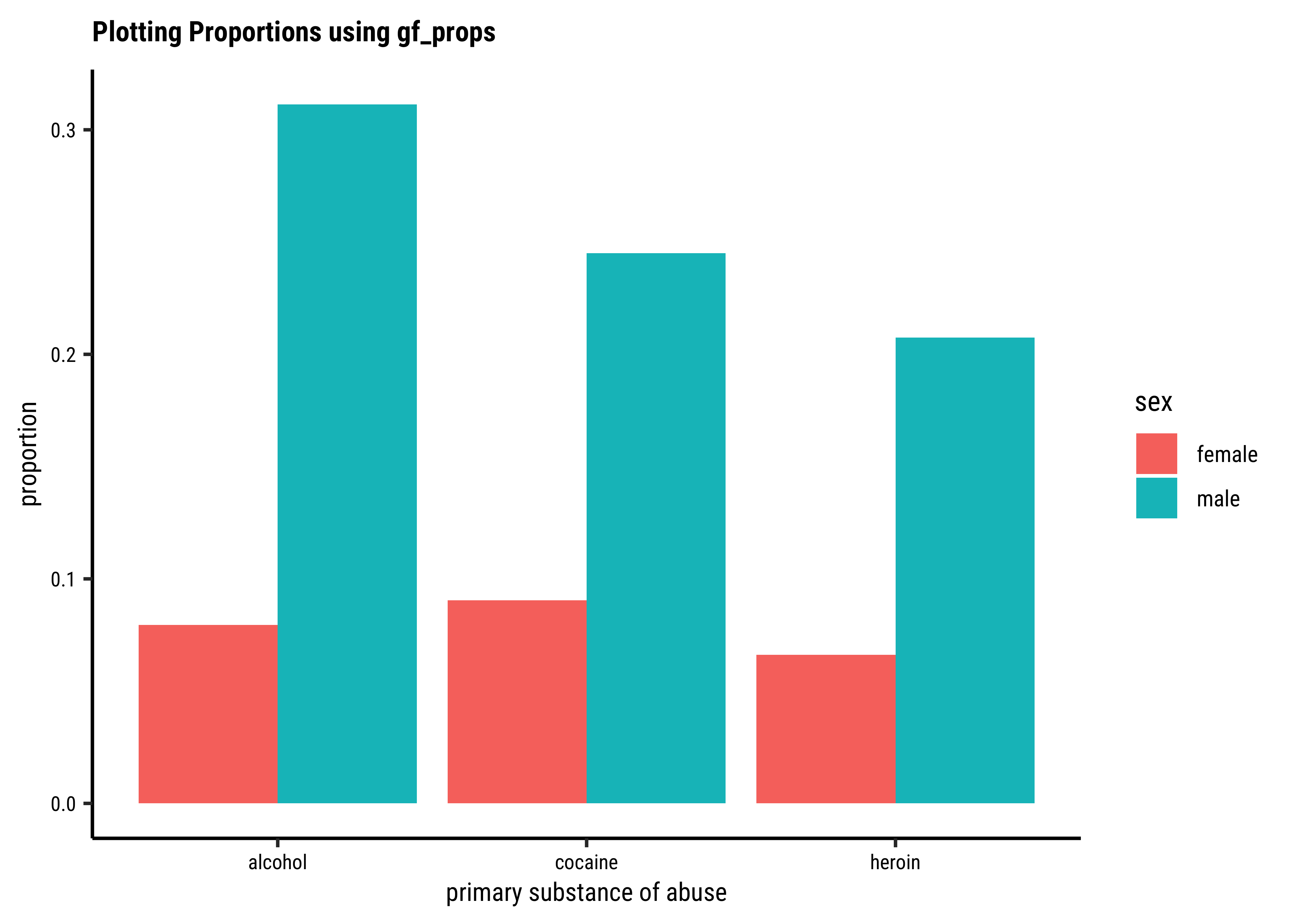
tidyplots::tidyplot(company,
colour = tip,
data = taxi_modified
) %>%
add_barstack_absolute() %>%
add_title("Plot 3B: Stacked Bar Chart") %>%
adjust_size(height = 50, width = 80, unit = "mm") %>%
adjust_x_axis(rotate_labels = 45)
tidyplots::tidyplot(company,
colour = tip,
data = taxi_modified
) %>%
add_barstack_relative() %>%
add_title("Plot 3C: Stacked Bar Chart") %>%
add_annotation_text(
text = "Proportions of Tippers per Company",
x = 4.25, y = 1.25
) %>%
adjust_size(height = 50, width = 80, unit = "mm") %>%
adjust_x_axis(title = "", rotate_labels = 45) %>%
adjust_y_axis(title = "Proportions") # Not happening??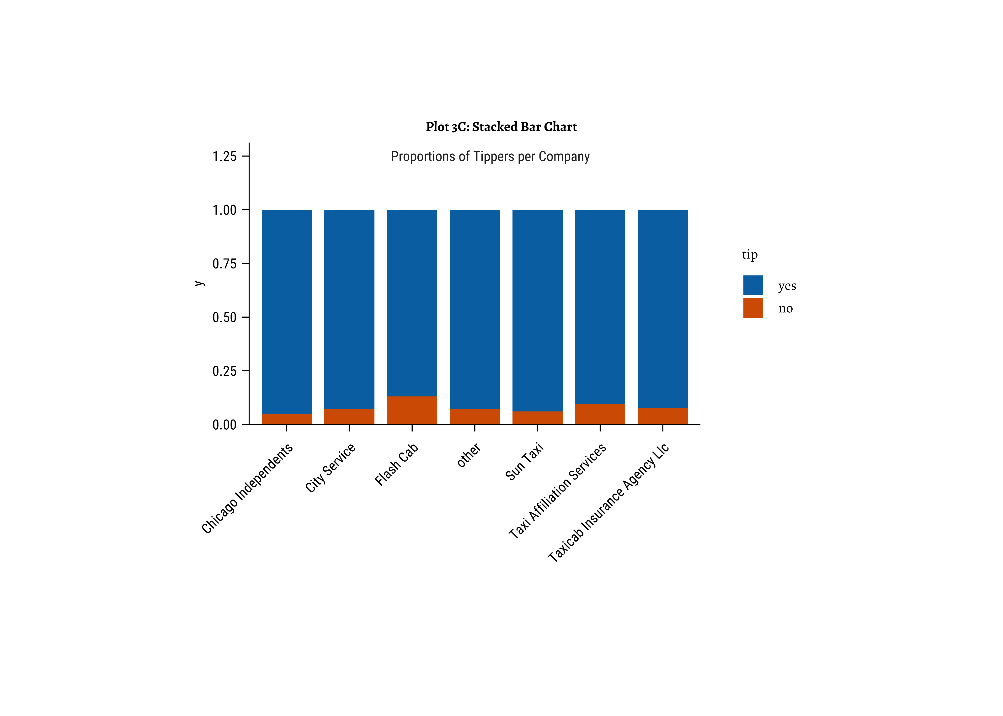
To be Coded!!
Business Insights-3
- Using
stack-ed,dodge-ed, andfill-ed in ggformula (andbars,absolute-stacked-bars, andrelative-stacked-barsin tidyplots) in bar plots gives us different ways of looking at the sets of counts; -
fill: gives us a per-group proportion of another Qual variable for a chosen Qual variable. This chart view is useful in Inference for Proportions; - Most cab
company-ies have similar usage, if you neglect theothercategory ofcompany; - Does seem that of all the
company-ies,tipsare not so good for theFlash Cabcompany. A driver issue? Or are the cars too old? Or don’t they offer service everywhere?
tip depend upon the distance, hour of day, and dow and month?
tip depend upon the distance, hour of day, and dow and month?

theme_set(new = theme_custom())
## This may be too busy a graph...
gf_bar(~ dow | hour, fill = ~tip, data = taxi_modified) %>%
gf_labs(
title = "Plot 4E: Counts of Tips by Hour and Day of Week",
subtitle = "Is this plot arrangement easy to grasp?"
) %>%
gf_refine(scale_fill_brewer(palette = "Set1"))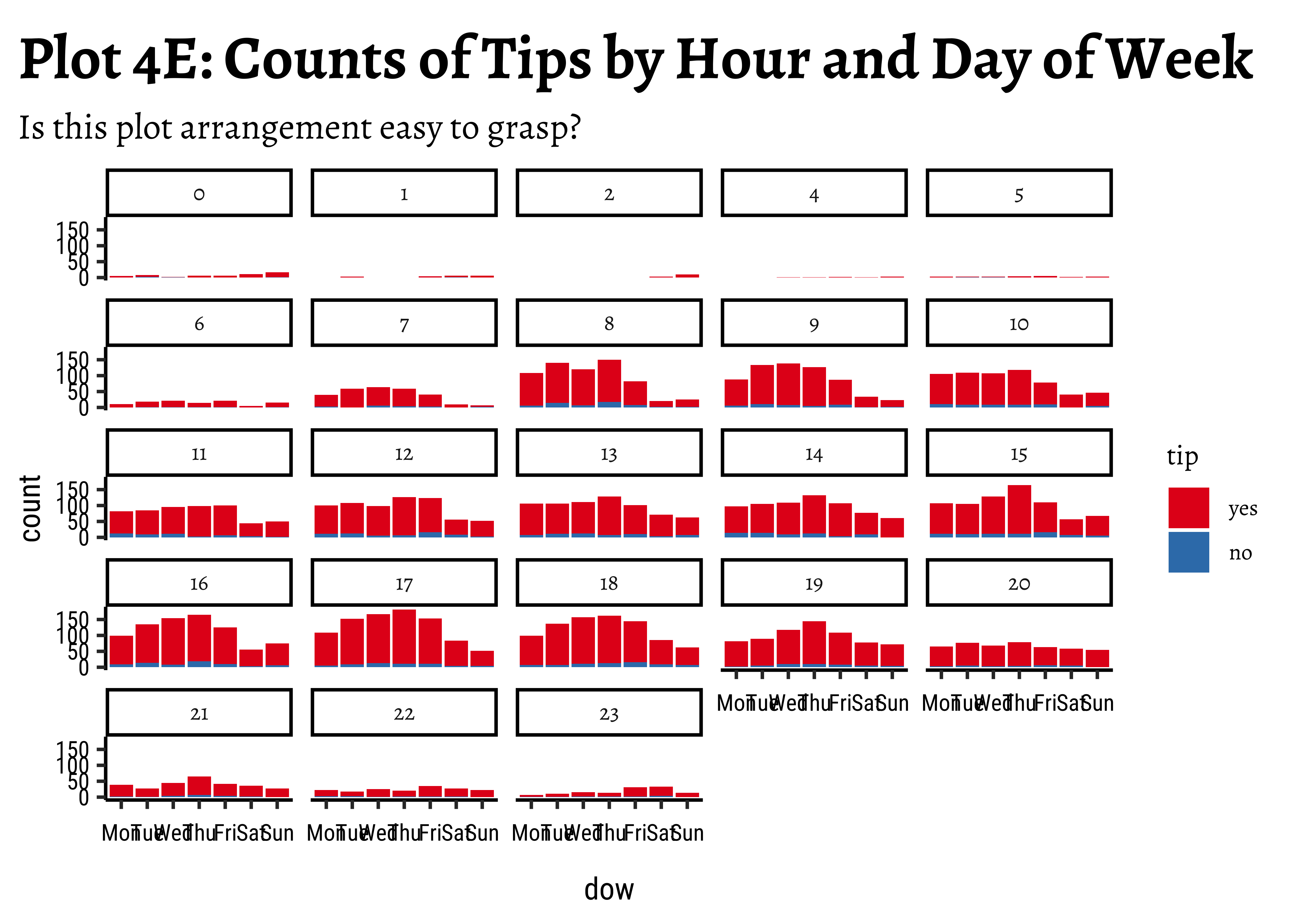
theme_set(new = theme_custom())
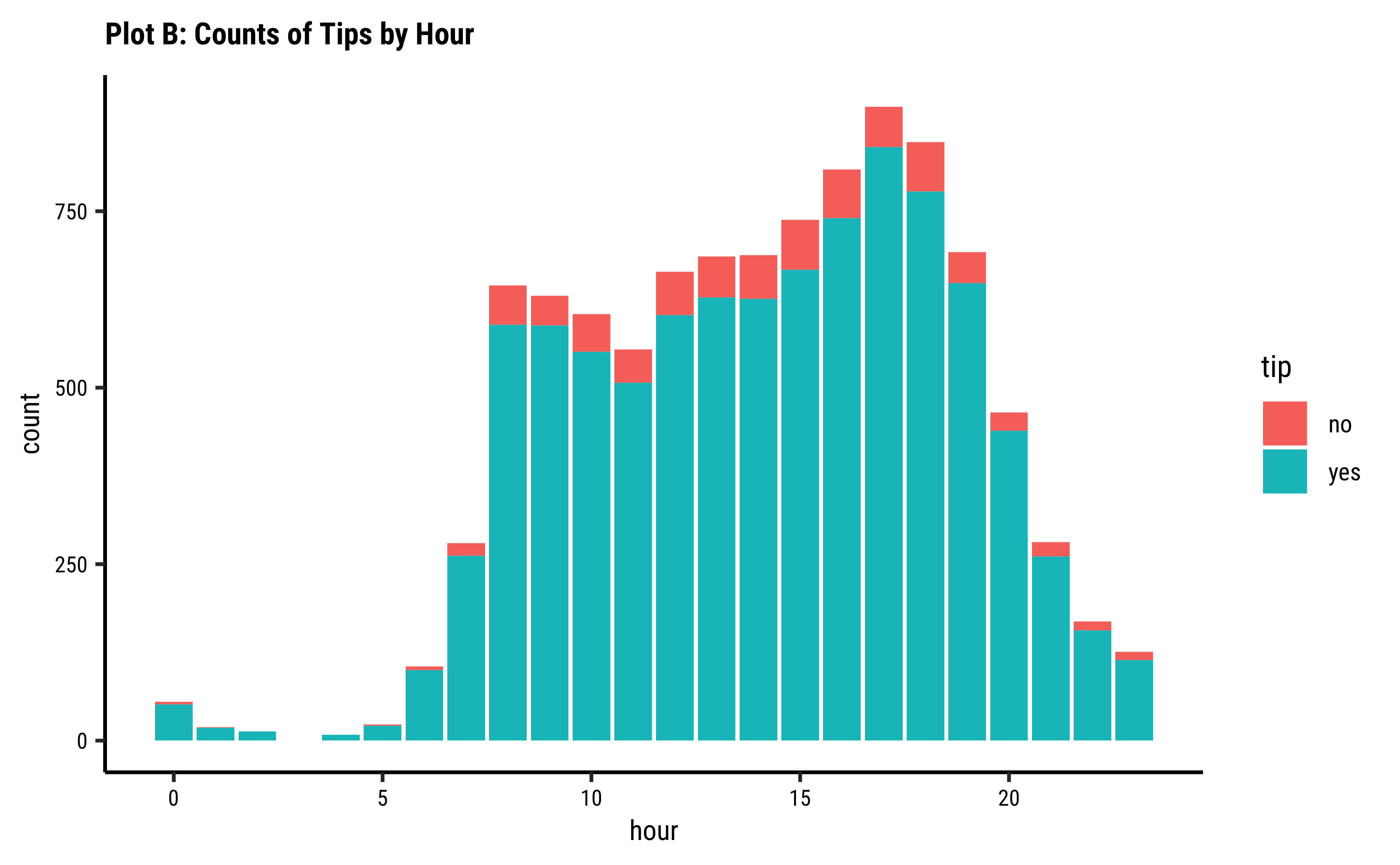
gf_bar(~hour, fill = ~tip, data = taxi_modified) %>%
gf_labs(title = "Plot 4A: Counts of Tips by Hour") %>%
gf_refine(scale_fill_brewer(palette = "Set1"))
##
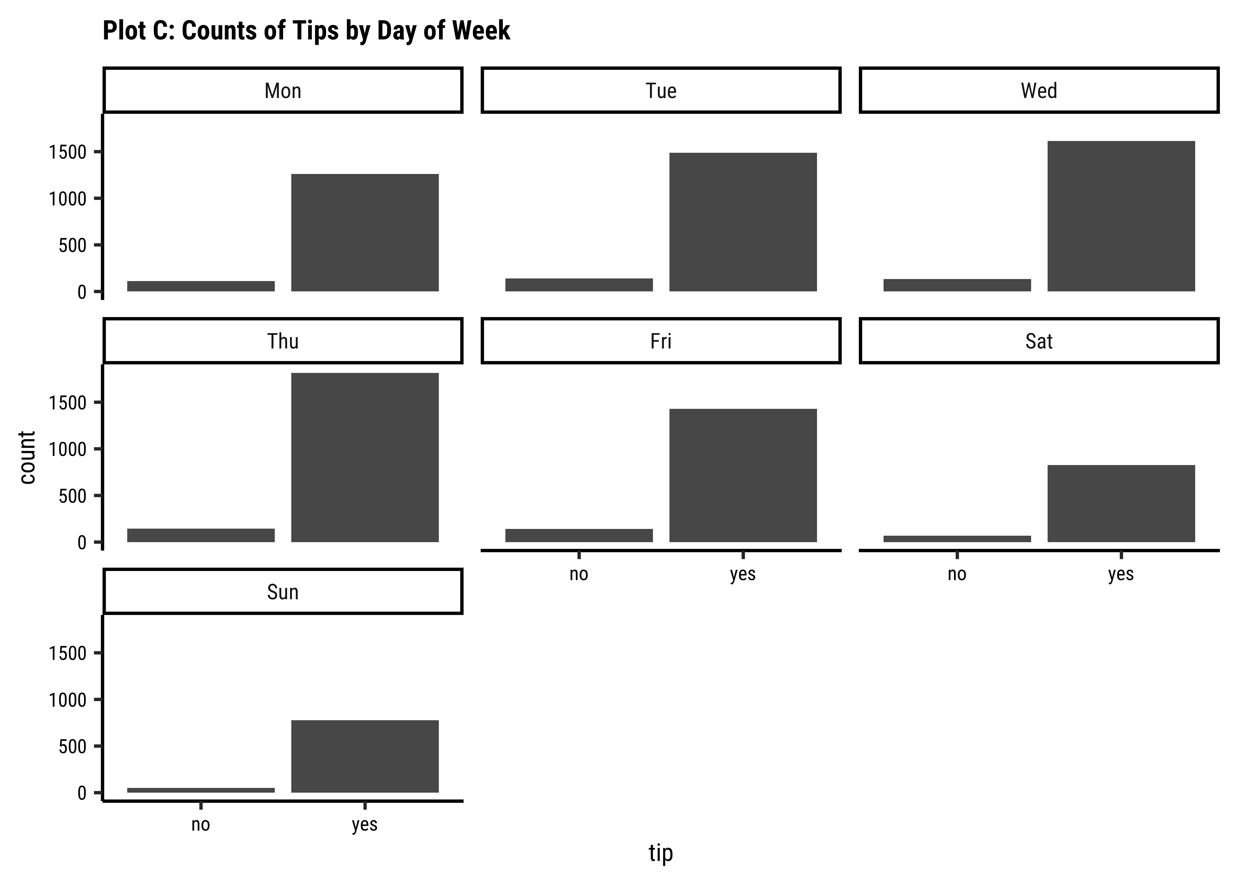
ggplot(taxi_modified) +
geom_bar(aes(x = dow, fill = tip)) +
labs(title = "Plot 4B: Counts of Tips by Day of Week") +
scale_fill_brewer(palette = "Set1")
##
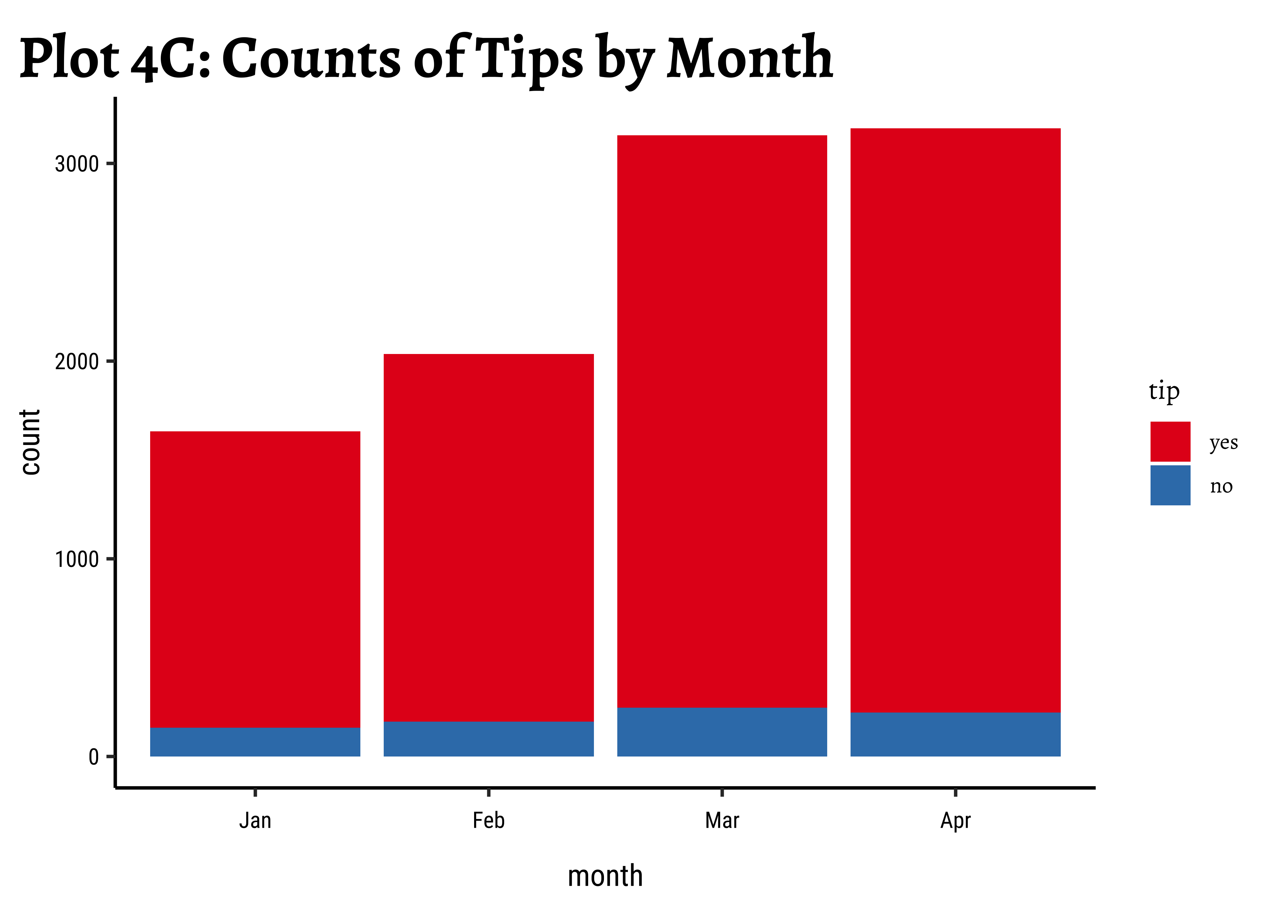
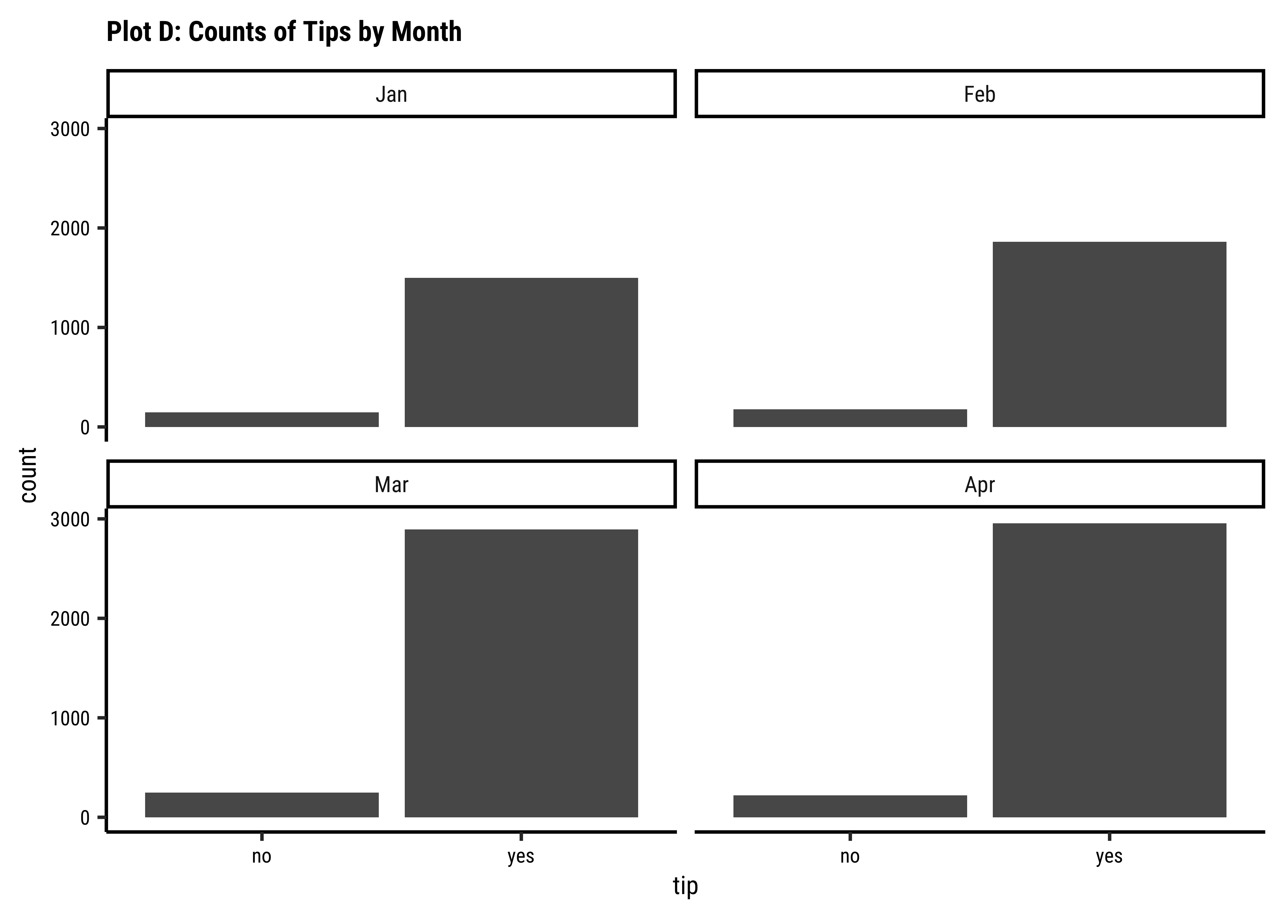
ggplot(taxi_modified) +
geom_bar(aes(x = month, fill = tip)) +
labs(title = "Plot 4C: Counts of Tips by Month") +
scale_fill_brewer(palette = "Set1")
##
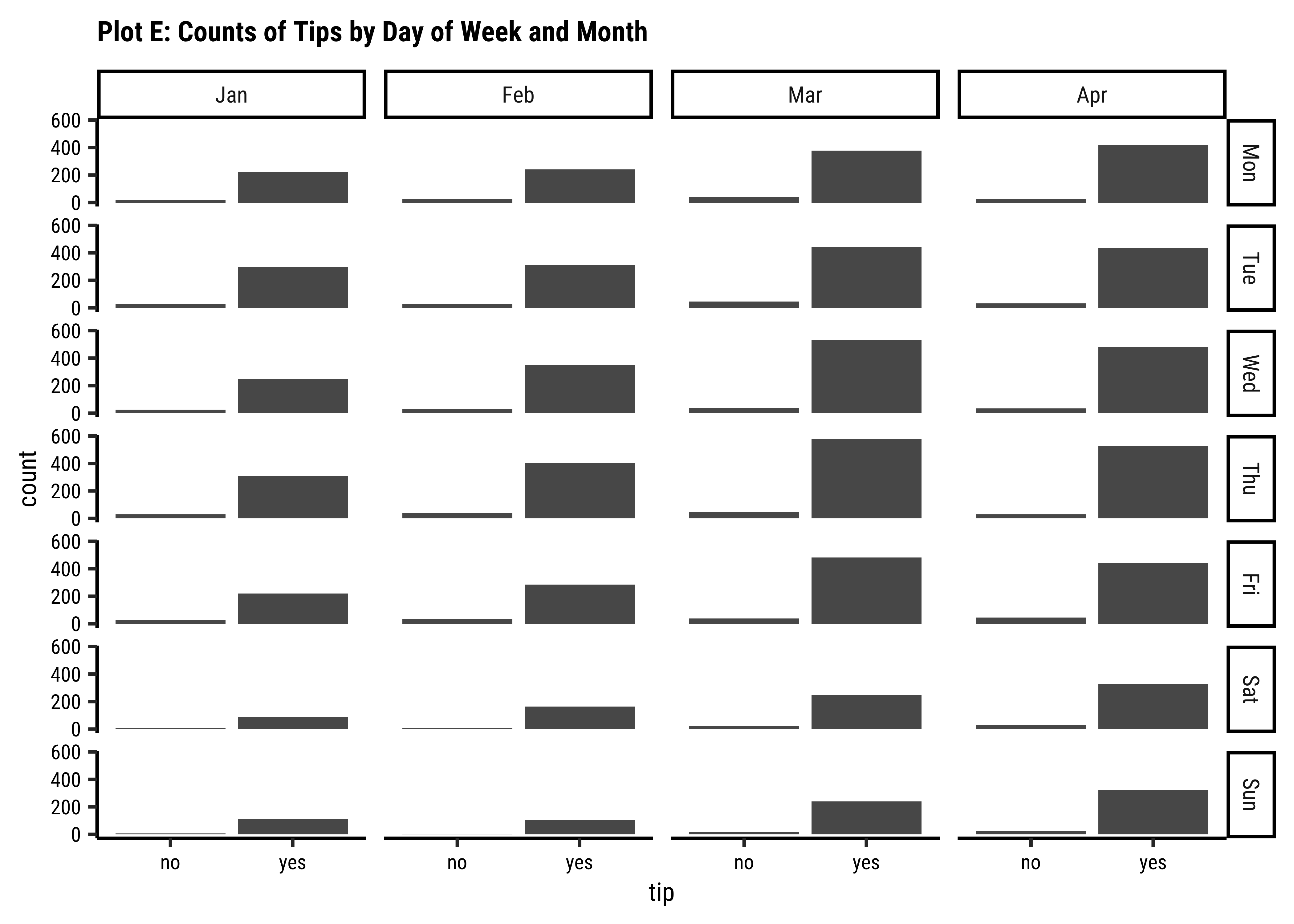
ggplot(taxi_modified) +
geom_bar(aes(x = month, fill = tip)) +
facet_wrap(~dow) +
labs(title = "Plot 4D: Counts of Tips by Day of Week and Month") +
scale_fill_brewer(palette = "Set1")
##
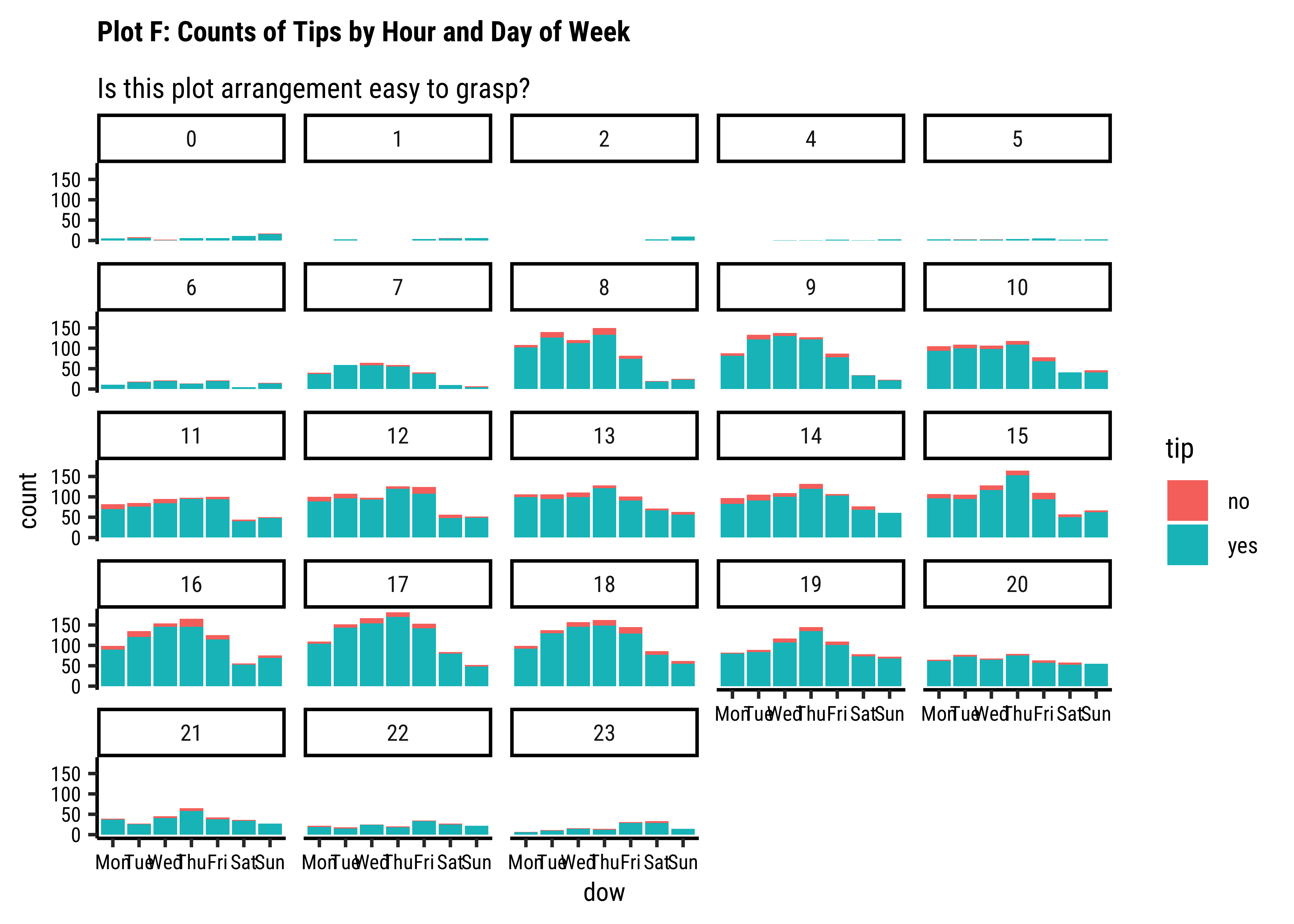
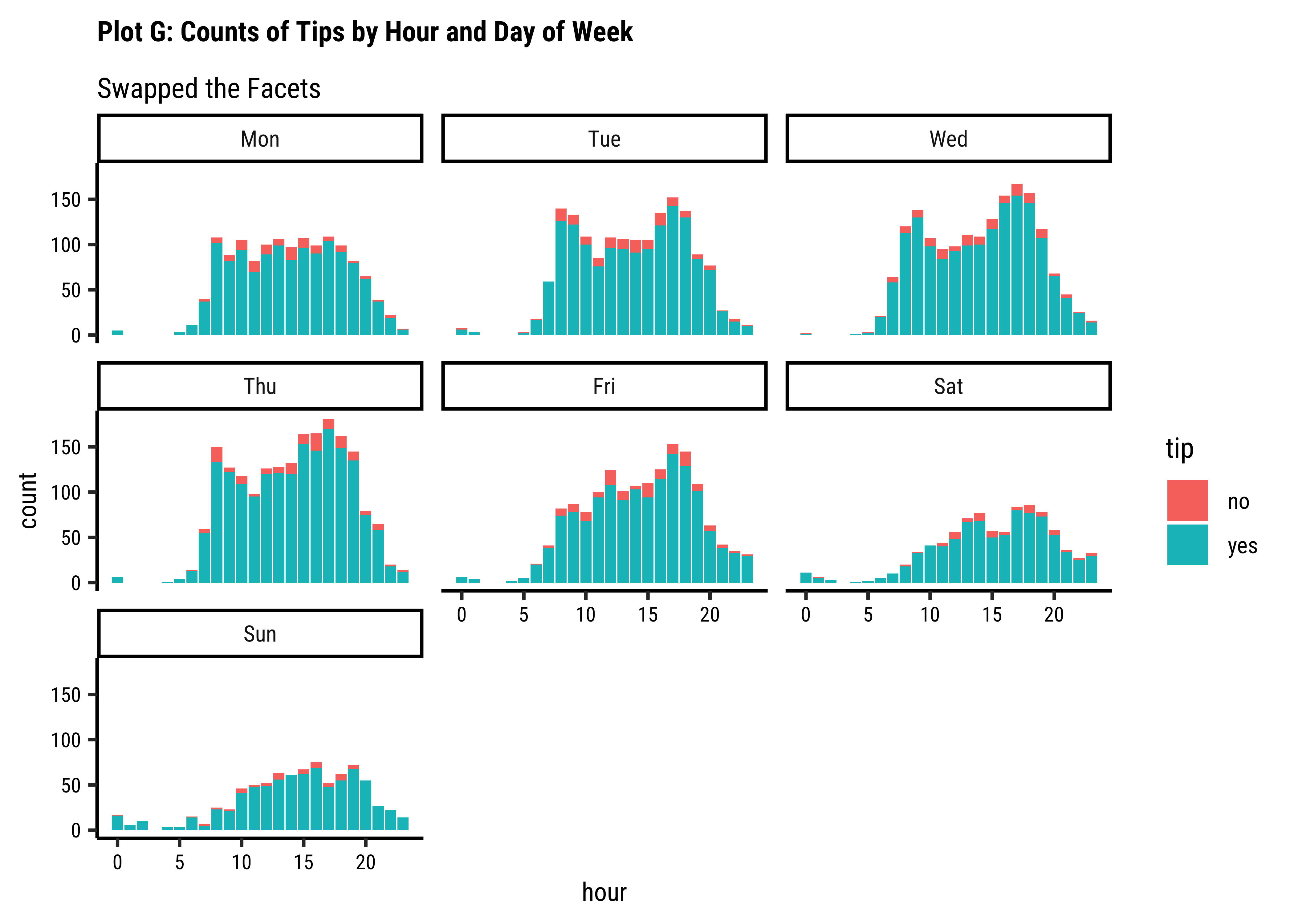
ggplot(taxi_modified) +
geom_bar(aes(x = dow, fill = tip)) +
facet_wrap(~hour) +
labs(
title = "Plot 4E: Counts of Tips by Hour and Day of Week",
subtitle = "Is this plot arrangement easy to grasp?"
) +
scale_fill_brewer(palette = "Set1")
##
ggplot(taxi_modified) +
geom_bar(aes(x = hour, fill = tip)) +
facet_wrap(~dow) +
labs(
title = "Plot 4F: Counts of Tips by Hour and Day of Week",
subtitle = "Swapped the Facets"
) +
scale_fill_brewer(palette = "Set1")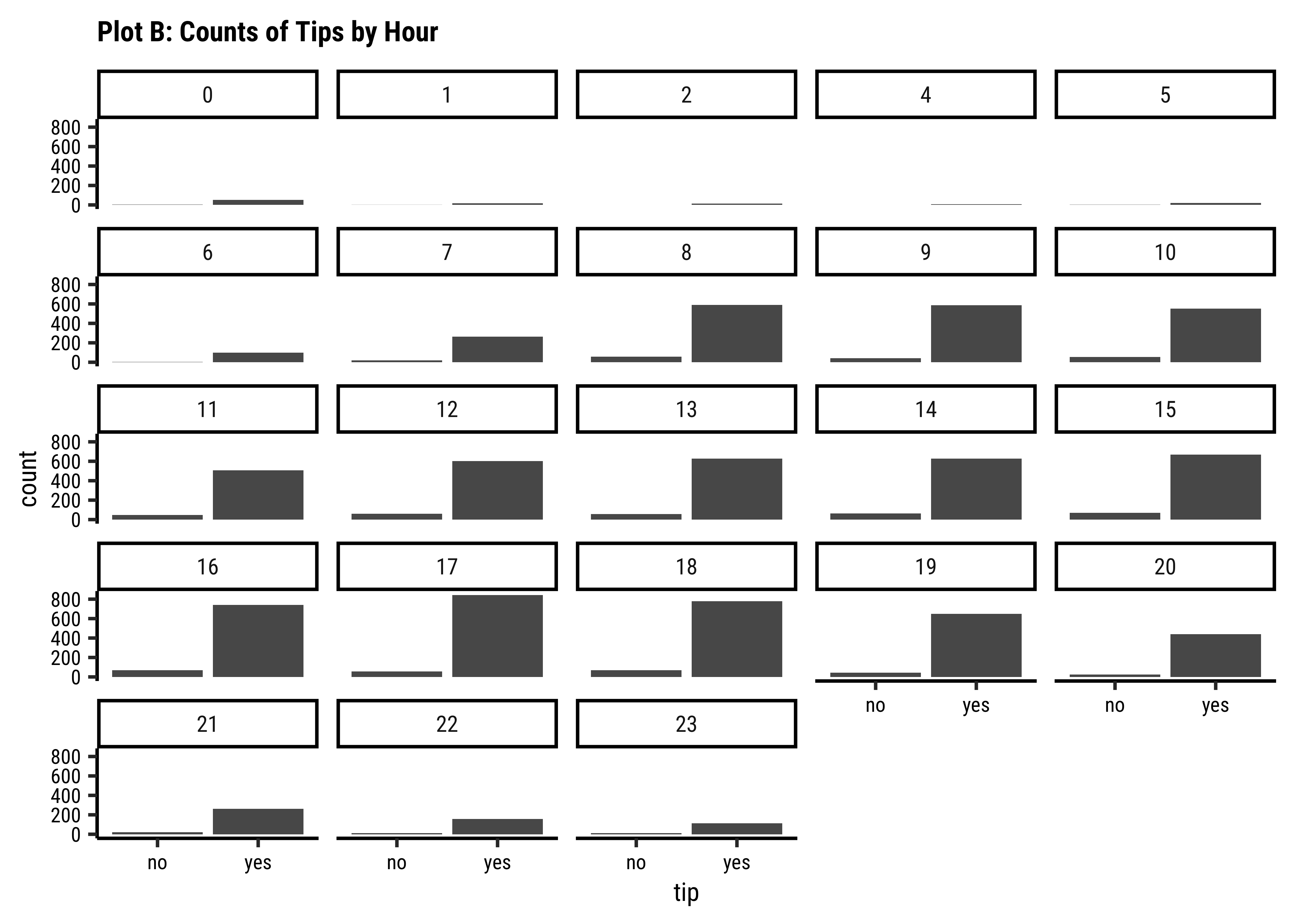
tidyplots::tidyplot(hour,
colour = tip,
data = taxi_modified
) %>%
add_count_bar() %>%
add_title("Plot 4A: Counts of Tips by Hour") %>%
adjust_size(height = 50, width = 80, unit = "mm") %>%
adjust_colors(colors_discrete_friendly)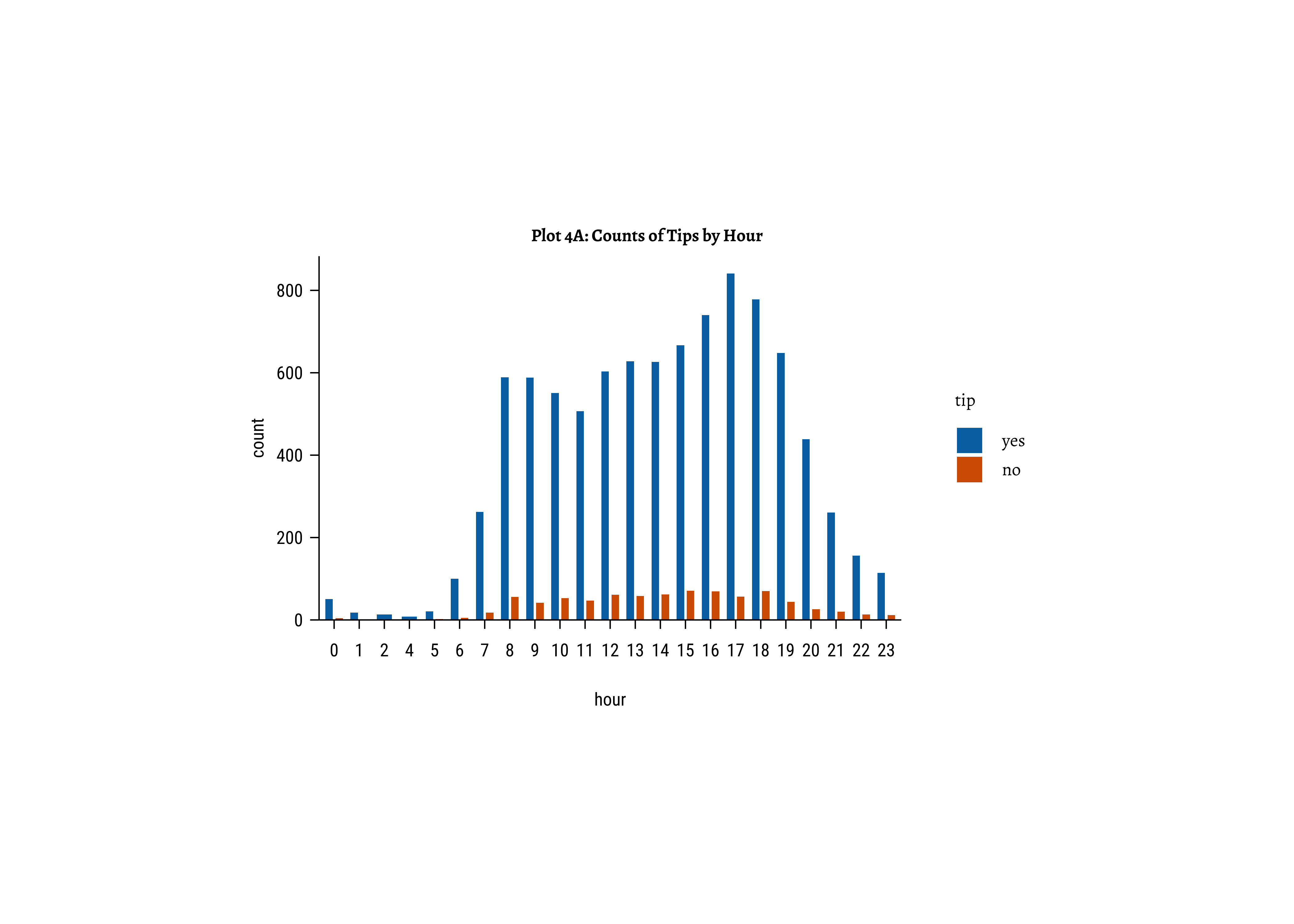
tidyplots::tidyplot(hour,
colour = tip,
data = taxi_modified
) %>%
add_barstack_absolute() %>%
add_title("Plot 4B: Counts of Tips by Hour") %>%
adjust_size(height = 50, width = 80, unit = "mm") %>%
adjust_colors(colors_discrete_friendly)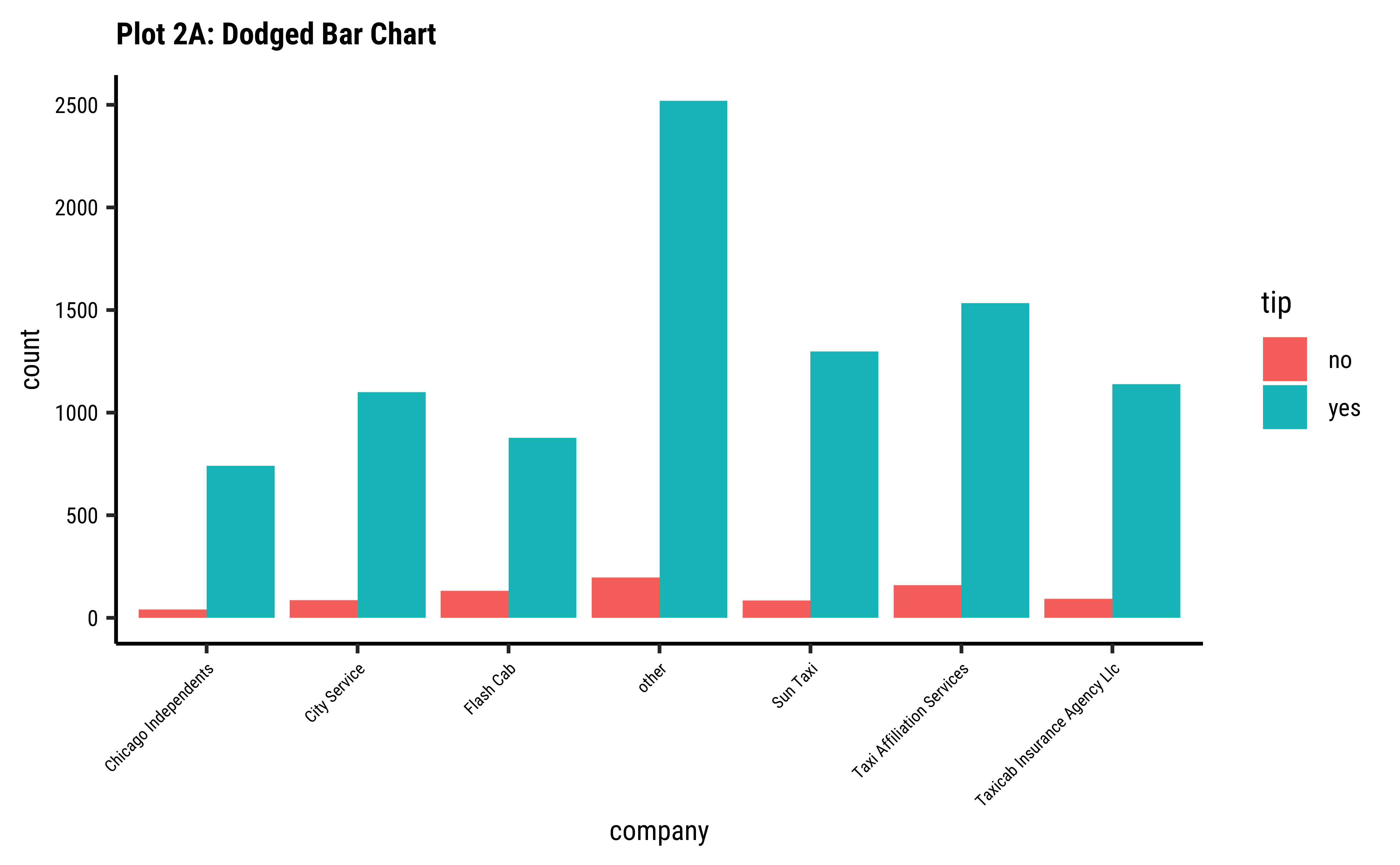
tidyplots::tidyplot(hour,
colour = tip,
data = taxi_modified
) %>%
add_barstack_relative() %>%
add_title("Plot 4C: Counts of Tips by Hour") %>%
adjust_size(height = 50, width = 80, unit = "mm") %>%
adjust_colors(colors_discrete_friendly)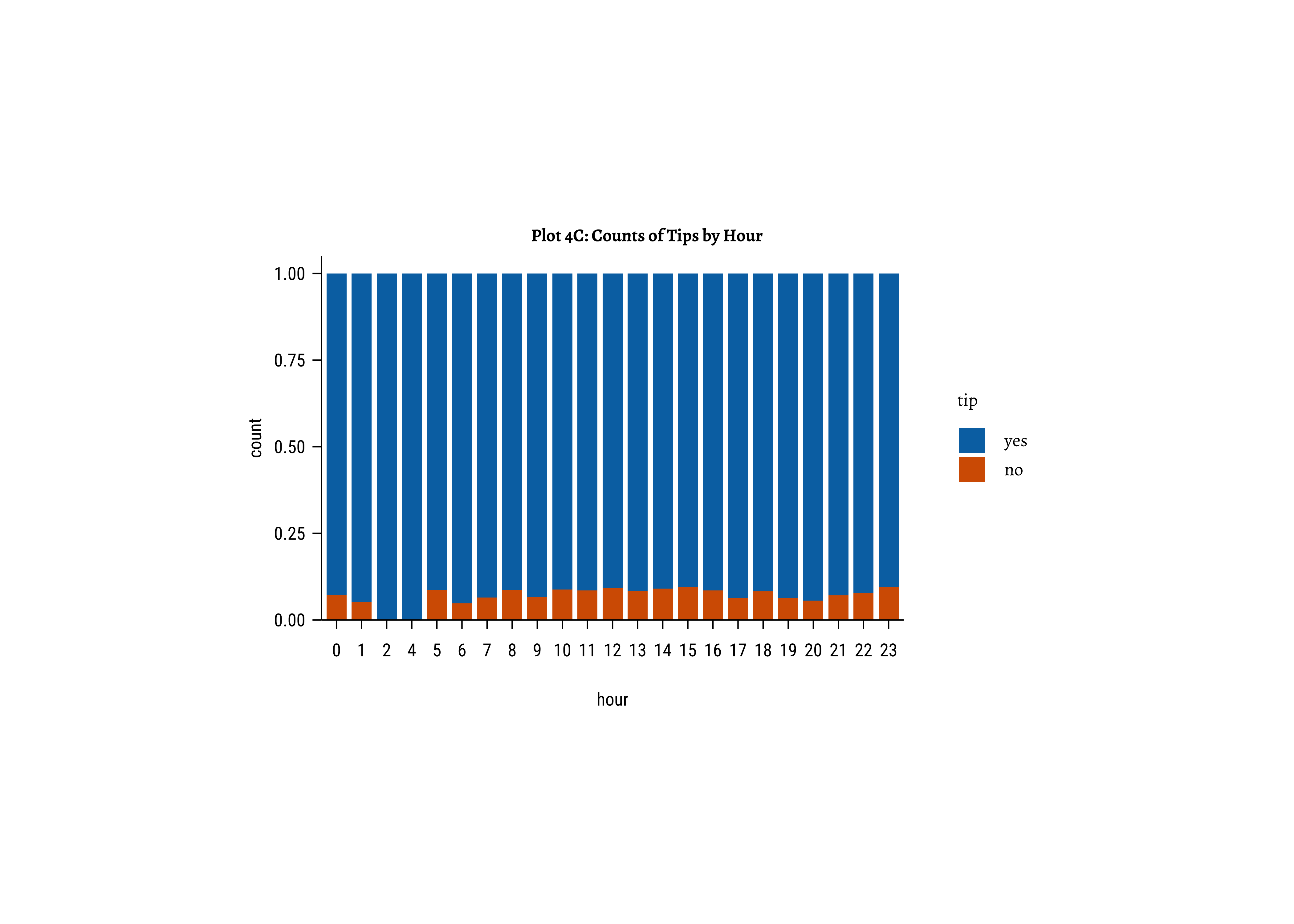
##
tidyplots::tidyplot(month,
colour = tip,
data = taxi_modified
) %>%
add_barstack_absolute() %>%
add_title("Plot 4D: Counts of Tips by Day of Week and Month") %>%
adjust_size(height = 50, width = 80, unit = "mm") %>%
adjust_colors(colors_discrete_friendly) %>%
split_plot(
by = dow,
ncol = 3, nrow = 3, guides = "collect"
)
##
tidyplots::tidyplot(dow,
colour = tip,
data = taxi_modified
) %>%
add_barstack_absolute() %>%
add_title("Plot 4D: Counts of Tips by Day of Week and Month") %>%
adjust_size(height = 50, width = 80, unit = "mm") %>%
adjust_colors(colors_discrete_friendly) %>%
adjust_x_axis(rotate_labels = 45) %>%
split_plot(
by = hour,
ncol = 3, nrow = 8, guides = "collect"
)
To be Coded.
Business Insights-4
- Note: We were using
fill = ~ tiphere! Why is that a good idea? -
tipsvshour: There are always more people whotipthan those who do not. Of course there are fewer trips during the early morning hours and the late night hours, based on the very small bar-pairs we see at those times -
tipsvsdow: Except for Sunday, thetipcount patterns (Yes/No) look similar across all days. -
tipsvsmonth: We have data for 4 months only. Again, thetipcount patterns (Yes/No) look similar across all months. Perhaps slightly fewer trips in Jan, when it is cold in Chicago and people may not go out much. -
tipsvsdowvsmonth: Very similar counts fortips(Yes/No) across day-of-week and month.
Note also that gf_bar/geom_bar takes only ONE variable (for the x-axis), whereas gf_col/geom_col needs both X and Y variables since it simply plots columns. Both are useful!
We have already seen gf_props in our two case studies above. Also check out gf_percents ! These are both very useful ggformula functions!
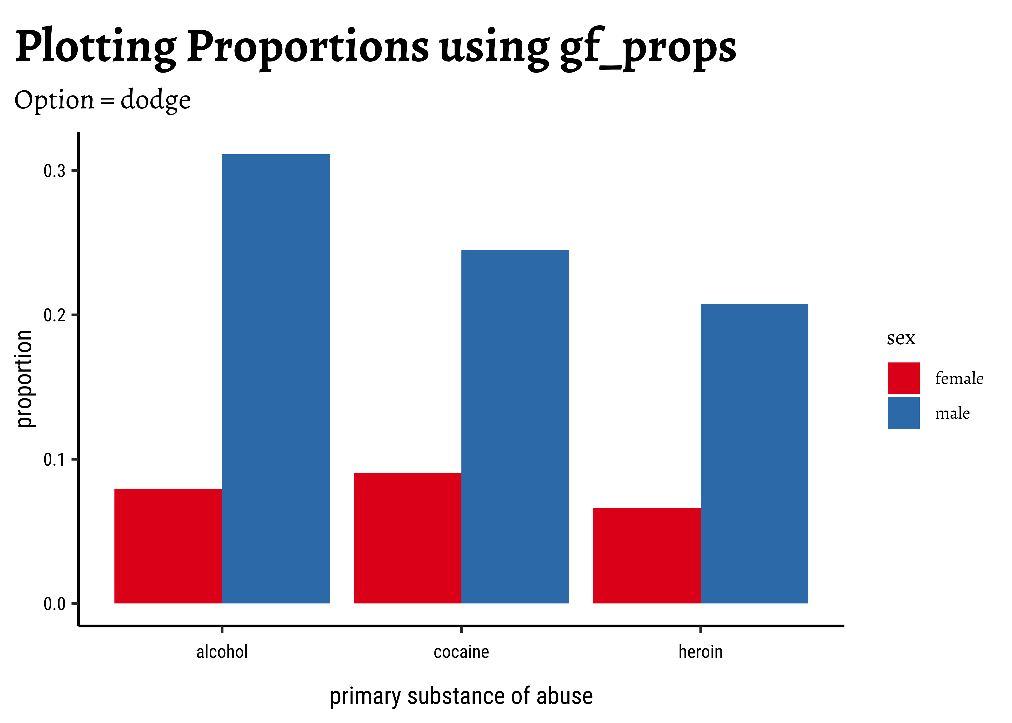
theme_set(new = theme_custom())
gf_percents(~substance,
data = mosaicData::HELPrct, fill = ~sex,
position = "dodge"
) %>%
gf_refine(
scale_y_continuous(
labels = scales::label_percent(scale = 1)
)
) %>%
gf_labs(title = "Plotting Percentages using gf_percents") %>%
gf_refine(scale_fill_brewer(palette = "Set1"))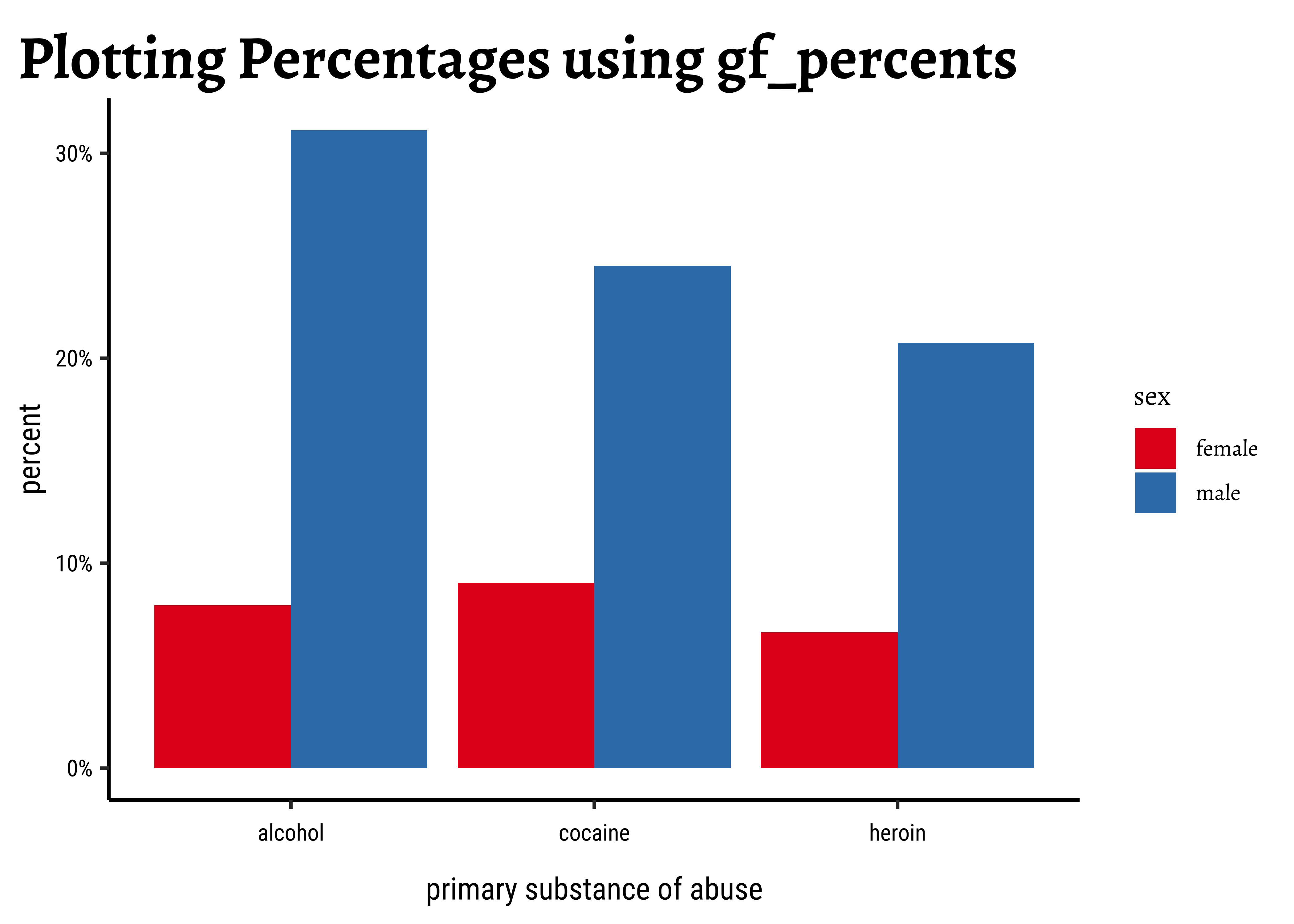
When we see situations such as this, where data has one or more Qual variables that are binary(Yes/No), we are always interested in whether these proportions of Yes/No are really different, or if we are just seeing the result of random chance. This is usually mechanized by a Stat Test called a Single Proportion Test or, when we have more than one, a Multiple Proportion Test.
Click on the Dataset Icon above, and unzip that archive. Try to make Bar plots with each of them, using one or more Qual variables.
A dataset from calmcode.io https://calmcode.io/datasets.html
- AiRbnb Price Data on the French Riviera:
- Apartment price vs ground living area:
- Fertility: This rather large and interesting Fertility related dataset from https://vincentarelbundock.github.io/Rdatasets/csv/AER/Fertility.csv