library(ggformula) # Formula based plots
library(mosaic) # Data inspection and Statistical Inference
library(broom) # Tidy outputs from Statistical Analyses
library(infer) # Statistical Inference, Permutation/Bootstrap
library(patchwork) # Arranging Plots
library(ggprism) # Interesting Categorical Axes
library(supernova) # Beginner-Friendly ANOVA Tables
library(paletteer) # Color Palettes
library(tidyverse) # Tidy Data ProcessingComparing Multiple Means with ANOVA
Abstract
ANOVA to investigate how frogspawn hatching time varies with temperature.
Plot Fonts and Theme
Show the Code
library(systemfonts)
library(showtext)
## Clean the slate
systemfonts::clear_local_fonts()
systemfonts::clear_registry()
##
showtext_opts(dpi = 96) # set DPI for showtext
sysfonts::font_add(
  family = "Alegreya",
  regular = "../../../../../../fonts/Alegreya-Regular.ttf",
  bold = "../../../../../../fonts/Alegreya-Bold.ttf",
  italic = "../../../../../../fonts/Alegreya-Italic.ttf",
  bolditalic = "../../../../../../fonts/Alegreya-BoldItalic.ttf"
)
Error in check_font_path(bold, "bold"): font file not found for 'bold' typeShow the Code
sysfonts::font_add(
  family = "Roboto Condensed",
  regular = "../../../../../../fonts/RobotoCondensed-Regular.ttf",
  bold = "../../../../../../fonts/RobotoCondensed-Bold.ttf",
  italic = "../../../../../../fonts/RobotoCondensed-Italic.ttf",
  bolditalic = "../../../../../../fonts/RobotoCondensed-BoldItalic.ttf"
)
showtext_auto(enable = TRUE) # enable showtext
##
theme_custom <- function() {
  font <- "Alegreya" # assign font family up front

  theme_classic(base_size = 14, base_family = font) %+replace% # replace elements we want to change

    theme(
      text = element_text(family = font), # set base font family

      # text elements
      plot.title = element_text( # title
        family = font, # set font family
        size = 24, # set font size
        face = "bold", # bold typeface
        hjust = 0, # left align
        margin = margin(t = 5, r = 0, b = 5, l = 0)
      ), # margin
      plot.title.position = "plot",
      plot.subtitle = element_text( # subtitle
        family = font, # font family
        size = 14, # font size
        hjust = 0, # left align
        margin = margin(t = 5, r = 0, b = 10, l = 0)
      ), # margin

      plot.caption = element_text( # caption
        family = font, # font family
        size = 9, # font size
        hjust = 1
      ), # right align

      plot.caption.position = "plot", # right align

      axis.title = element_text( # axis titles
        family = "Roboto Condensed", # font family
        size = 12
      ), # font size

      axis.text = element_text( # axis text
        family = "Roboto Condensed", # font family
        size = 9
      ), # font size

      axis.text.x = element_text( # margin for axis text
        margin = margin(5, b = 10)
      )

      # since the legend often requires manual tweaking
      # based on plot content, don't define it here
    )
}
Show the Code
```{r}
#| cache: false
#| code-fold: true
## Set the theme
theme_set(new = theme_custom())

## Use available fonts in ggplot text geoms too!
update_geom_defaults(geom = "text", new = list(
  family = "Roboto Condensed",
  face = "plain",
  size = 3.5,
  color = "#2b2b2b"
))
```
Suppose we have three sales strategies on our website, to sell a certain product, say men’s shirts. We have observations of customer website interactions over several months. How do we know which strategy makes people buy the fastest ?
If there is a University course that is offered in parallel in three different classrooms, is there a difference between the average marks obtained by students in each of the classrooms?
In each case we have a set of Quant observations in each Qual category: Interaction Time vs Sales Strategy in the first example, and Student Marks vs Classroom in the second. We can take mean scores in each category and decide to compare them. How do we make the comparisons? One way would be to compare them pair-wise, doing as many t-tests as there are pairs. But with this rapidly becomes intractable and also dangerous: with increasing number of groups, the number of mean-comparisons becomes very large
In this tutorial, we will compare the Hatching Time of frog spawn1, at three different lab temperatures.
In this tutorial, our research question is:
Research Question
Based on the sample dataset at hand, how does frogspawn hatching time vary with different temperature settings?
Download the data by clicking the button below.
Data Folder
Save the CSV in a subfolder titled “data” inside your R work folder.
frogs_orig <- read_csv("data/frogs.csv")
frogs_origFrogspawn sample id <dbl> | Temperature13 <dbl> | Temperature18 <dbl> | Temperature25 <dbl> | |
|---|---|---|---|---|
| 1 | 24 | NA | NA | |
| 2 | NA | 21 | NA | |
| 3 | NA | NA | 18 | |
| 4 | 26 | NA | NA | |
| 5 | NA | 22 | NA | |
| 6 | NA | NA | 14 | |
| 7 | 27 | NA | NA | |
| 8 | NA | 22 | NA | |
| 9 | NA | NA | 15 | |
| 10 | 27 | NA | NA |
Our response variable is the hatching Time. Our explanatory variable is a factor, Temperature, with 3 levels: 13°C, 18°C and 25°C. Different samples of spawn were subject to each of these temperatures respectively.
The data is in wide-format, with a separate column for each Temperature, and a common column for Sample ID. This is good for humans, but poor for a computer: there are NA entries since not all samples of spawn can be subject to all temperatures. (E.g. Sample ID #1 was maintained at 13°C, and there are NAs in the other two columns, which we don’t need).
We will first stack up the Temperature columns into a single column, separate that into pieces and then retain just the number part (13, 18, 25), getting rid of the word Temperature from the column titles. Then the remaining numerical column with temperatures (13, 18, 25) will be converted into a factor.
We will use pivot_longer()and separate_wider_regex() to achieve this. [See this animation for pivot_longer(): https://haswal.github.io/pivot/ ]
frogs_orig %>%
  pivot_longer(
    .,
    cols = starts_with("Temperature"),
    cols_vary = "fastest",
    # new in pivot_longer
    names_to = "Temp",
    values_to = "Time"
  ) %>%
  drop_na() %>%
  ##
  separate_wider_regex(
    cols = Temp,
    # knock off the unnecessary "Temperature" word
    # Just keep the digits thereafter
    patterns = c("Temperature", TempFac = "\\d+"),
    cols_remove = TRUE
  ) %>%
  # Convert Temp into TempFac, a 3-level factor
  mutate(TempFac = factor(
    x = TempFac,
    levels = c(13, 18, 25),
    labels = c("13", "18", "25")
  )) %>%
  rename("Id" = `Frogspawn sample id`) -> frogs_long
frogs_long
##
frogs_long %>% count(TempFac)Id <dbl> | TempFac <fct> | Time <dbl> | ||
|---|---|---|---|---|
| 1 | 13 | 24 | ||
| 2 | 18 | 21 | ||
| 3 | 25 | 18 | ||
| 4 | 13 | 26 | ||
| 5 | 18 | 22 | ||
| 6 | 25 | 14 | ||
| 7 | 13 | 27 | ||
| 8 | 18 | 22 | ||
| 9 | 25 | 15 | ||
| 10 | 13 | 27 |
TempFac <fct> | n <int> | |||
|---|---|---|---|---|
| 13 | 20 | |||
| 18 | 20 | |||
| 25 | 20 |
So we have cleaned up our data and have 20 samples for Hatching Time per TempFac setting.
Let us plot some histograms and boxplots of Hatching Time:
# Set graph theme
theme_set(new = theme_custom())
##
gf_histogram(~Time,
  fill = ~TempFac,
  data = frogs_long, alpha = 0.5
) %>%
  gf_vline(xintercept = ~ mean(Time)) %>%
  gf_labs(
    title = "Histograms of Hatching Time Distributions vs Temperature",
    x = "Hatching Time", y = "Count"
  ) %>%
  gf_text(7 ~ (mean(Time) + 2),
    label = "Overall Mean"
  ) %>%
  gf_refine(
    scale_fill_paletteer_d("ggthemes::colorblind"),
    guides(fill = guide_legend(title = "Temperature level (°C)"))
  )
# Set graph theme
theme_set(new = theme_custom())
##
gf_boxplot(
data = frogs_long,
Time ~ TempFac,
fill = ~TempFac,
alpha = 0.5
) %>%
gf_vline(xintercept = ~ mean(Time)) %>%
gf_labs(
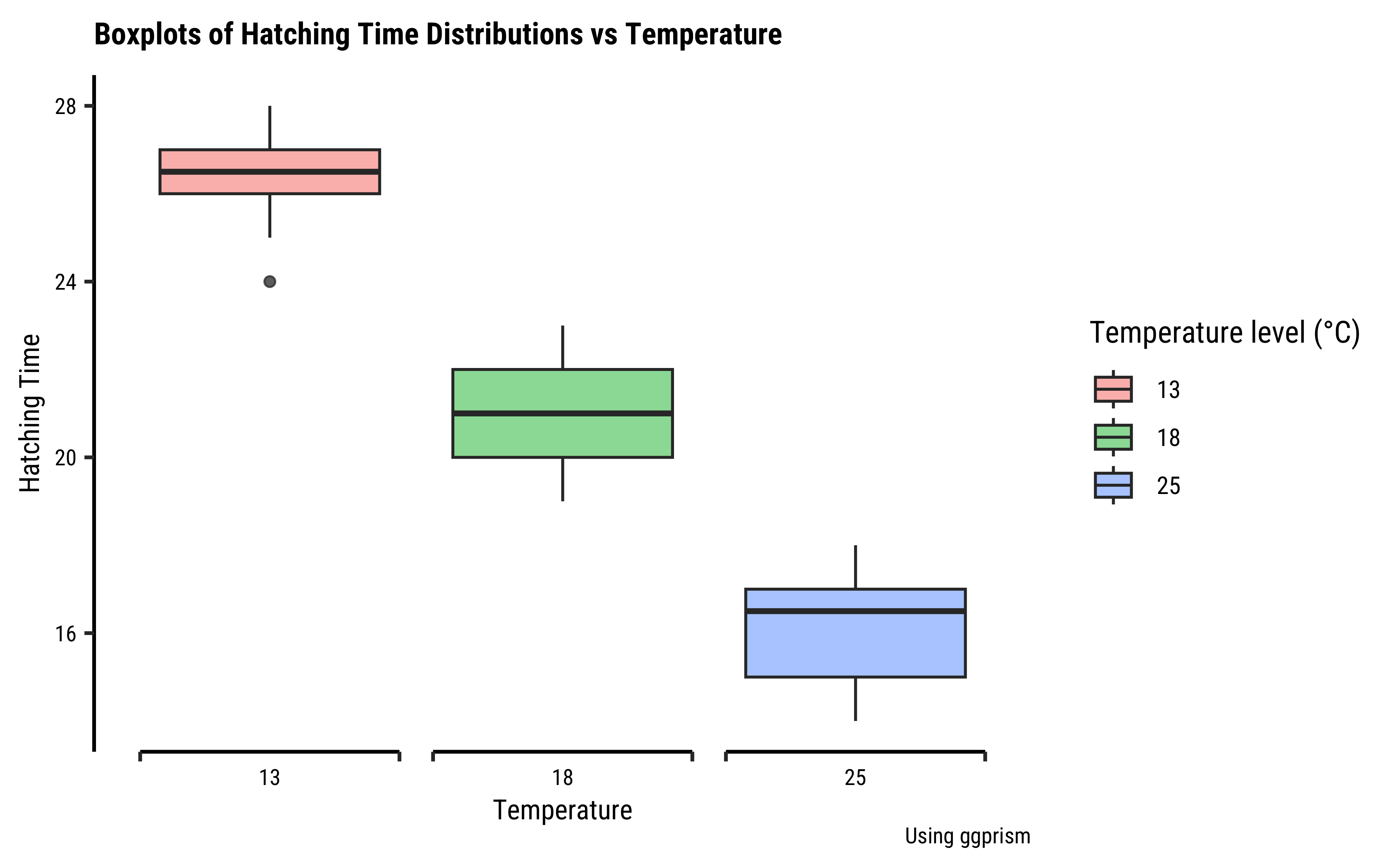
title = "Boxplots of Hatching Time Distributions vs Temperature",
x = "Temperature", y = "Hatching Time",
caption = "Using ggprism"
) %>%
gf_refine(
scale_fill_paletteer_d("ggthemes::colorblind"),
scale_x_discrete(guide = "prism_bracket"),
guides(fill = guide_legend(title = "Temperature level (°C)"))
)
The histograms look well separated and the box plots also show very little overlap. So we can reasonably hypothesize that Temperature has a significant effect on Hatching Time.
Let’s go ahead with our ANOVA test.
We will first execute the ANOVA test with code and evaluate the results. Then we will do an intuitive walkthrough of the process and finally, hand-calculate entire analysis for clear understanding. For now, a little faith!
R offers a very simple command aov to execute an ANOVA test: Note the familiar formula of stating the variables:
frogs_anova <- aov(Time ~ TempFac, data = frogs_long)This creates an ANOVA model object, called frogs_anova. We can examine the ANOVA model object best with a package called supernova2:
# library(supernova)
# Set graph theme
theme_set(new = theme_custom())
#
supernova::pairwise(frogs_anova,
  correction = "Bonferroni", # Try "Tukey"
  alpha = 0.05, # 95% CI calculation
  var_equal = TRUE, # We'll see
  plot = TRUE
)
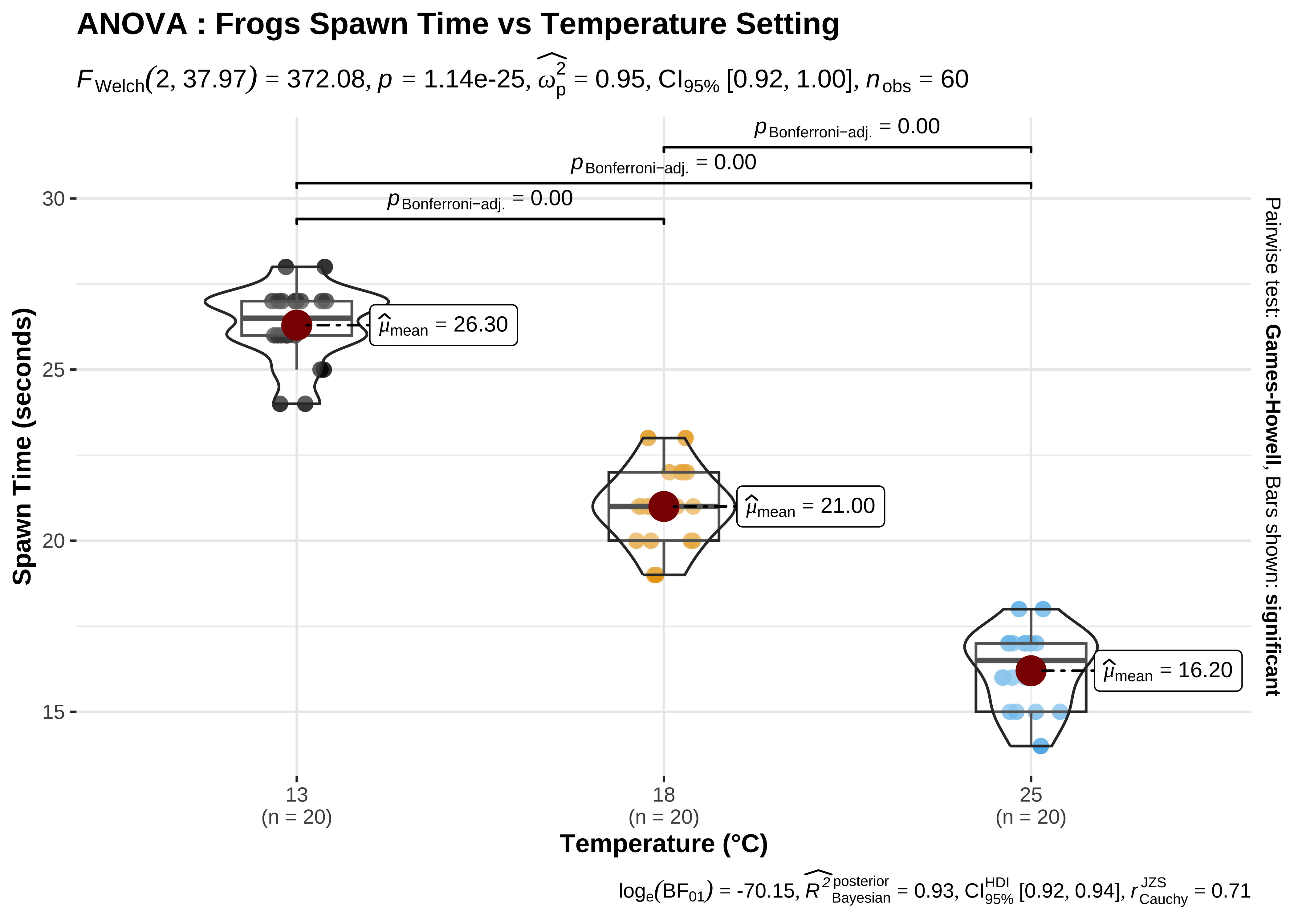
group_1 group_2 diff pooled_se t df lower upper p_adj
<chr> <chr> <dbl> <dbl> <dbl> <int> <dbl> <dbl> <dbl>
1 18 13 -5.300 0.257 -20.608 57 -5.861 -4.739 .0000
2 25 13 -10.100 0.257 -39.272 57 -10.661 -9.539 .0000
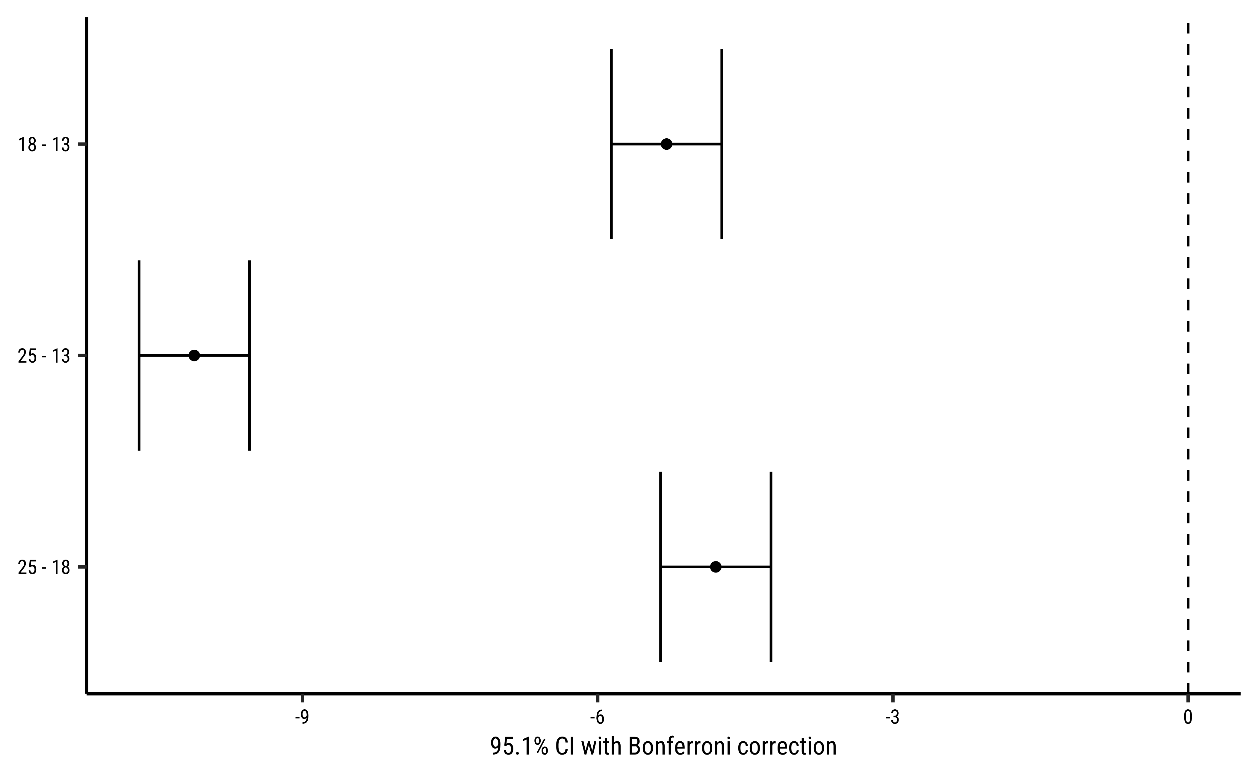
3 25 18 -4.800 0.257 -18.664 57 -5.361 -4.239 .0000This table + error-bar plot gives us a clear comparison between each pair of the three groups of observations defined by TempFac. The differences in spawn hatching Time between each pair of TempFac settings are given by the diff column. Also shown are the confidence intervals for each of these differences (none of which include p-values for each of these differences is also negligible. Thus we can conclude that the effect of temperature on hatching time is significant.
Note
To find which specific value of TempFac has the most effect will require pairwise comparison of the group means, using a standard t-test. The confidence level for such repeated comparisons will need what is called Bonferroni correction3 to prevent us from detecting a significant (pair-wise) difference simply by chance. To do this we take supernova::pairwise() function did this for us very neatly!
There are also other ways, such as the “Tukey correction” for multiple tests.
All that is very well, but what is happening under the hood of the aov() command?
Consider a data set with a single Quant and a single Qual variable. The Qual variable has two levels, the Quant data has 20 observations per Qual level.
index <int> | qual <chr> | quant <dbl> | ||
|---|---|---|---|---|
| 1 | A | 2.7419169 | ||
| 2 | A | -1.1293963 | ||
| 3 | A | 0.7262568 | ||
| 4 | A | 1.2657252 | ||
| 5 | A | 0.8085366 | ||
| 6 | A | -0.2122490 | ||
| 7 | A | 3.0230440 | ||
| 8 | A | -0.1893181 | ||
| 9 | A | 4.0368474 | ||
| 10 | A | -0.1254282 |
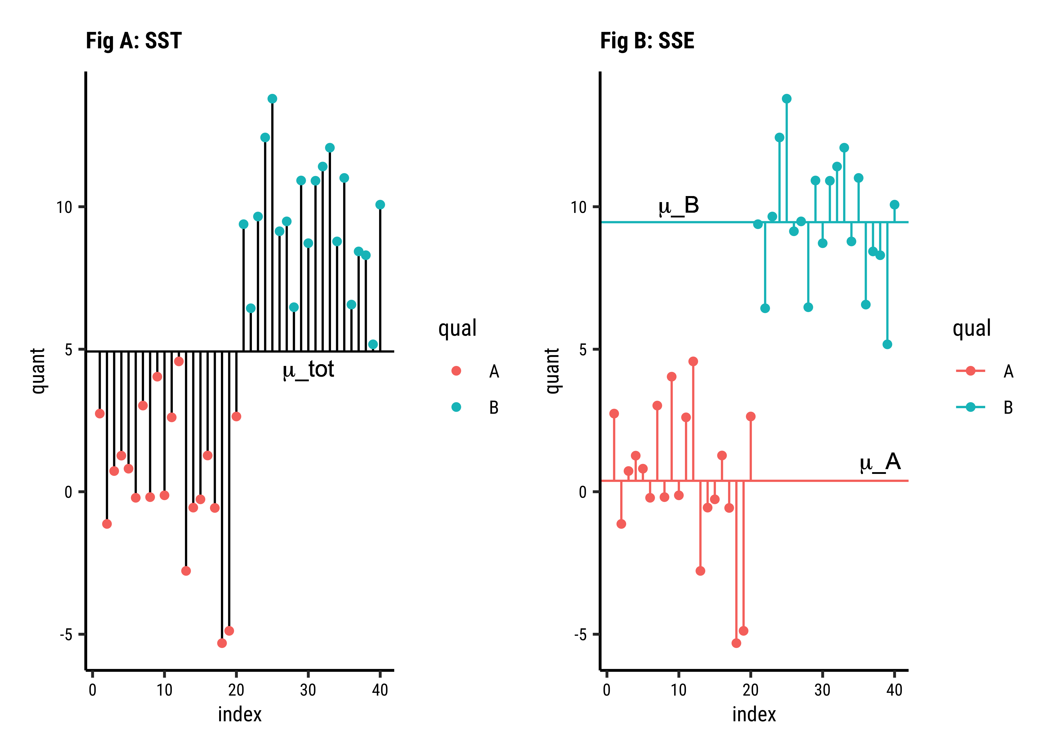
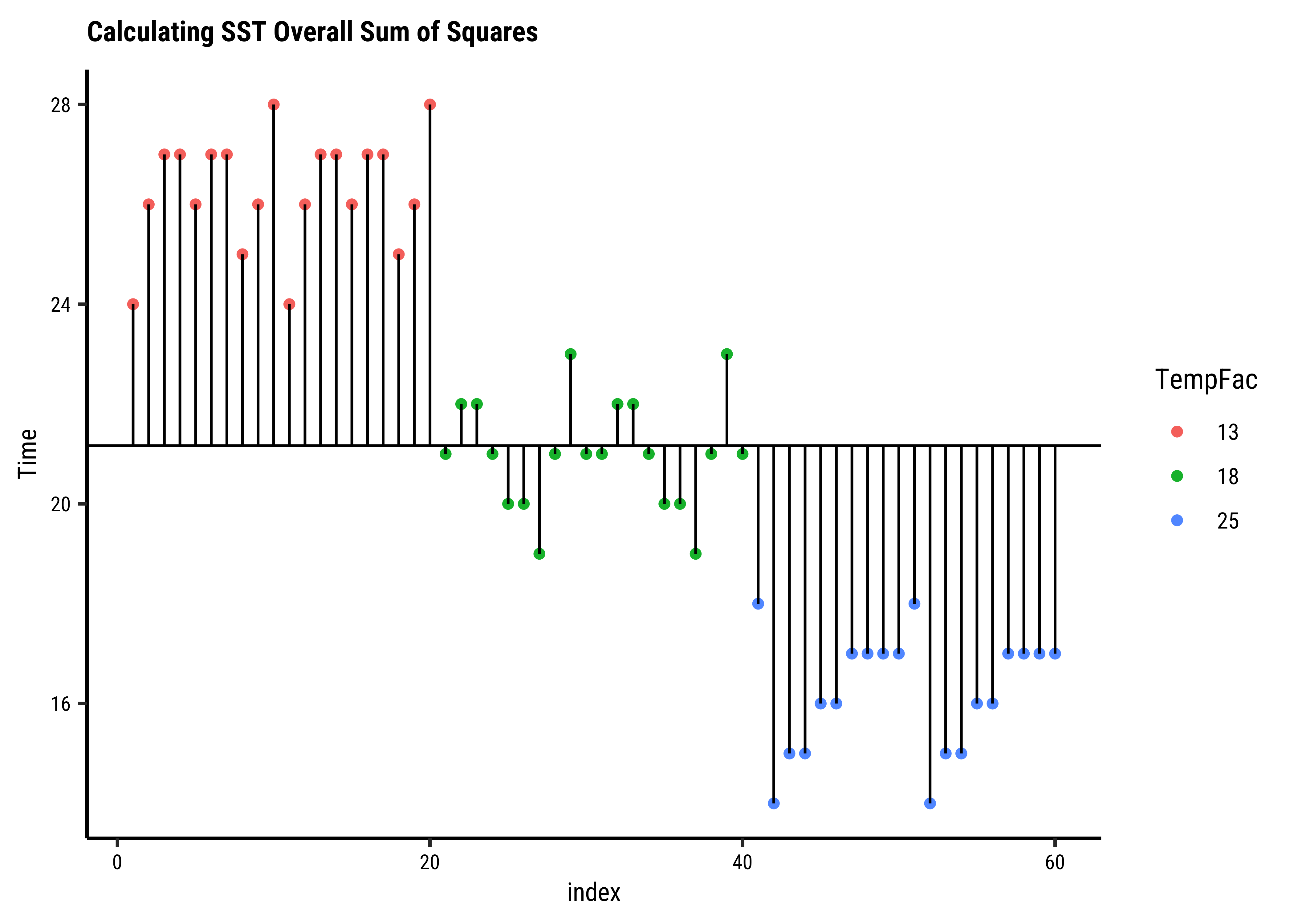
All Data: In Fig A, the horizontal black line is the overall mean of quant, denoted as
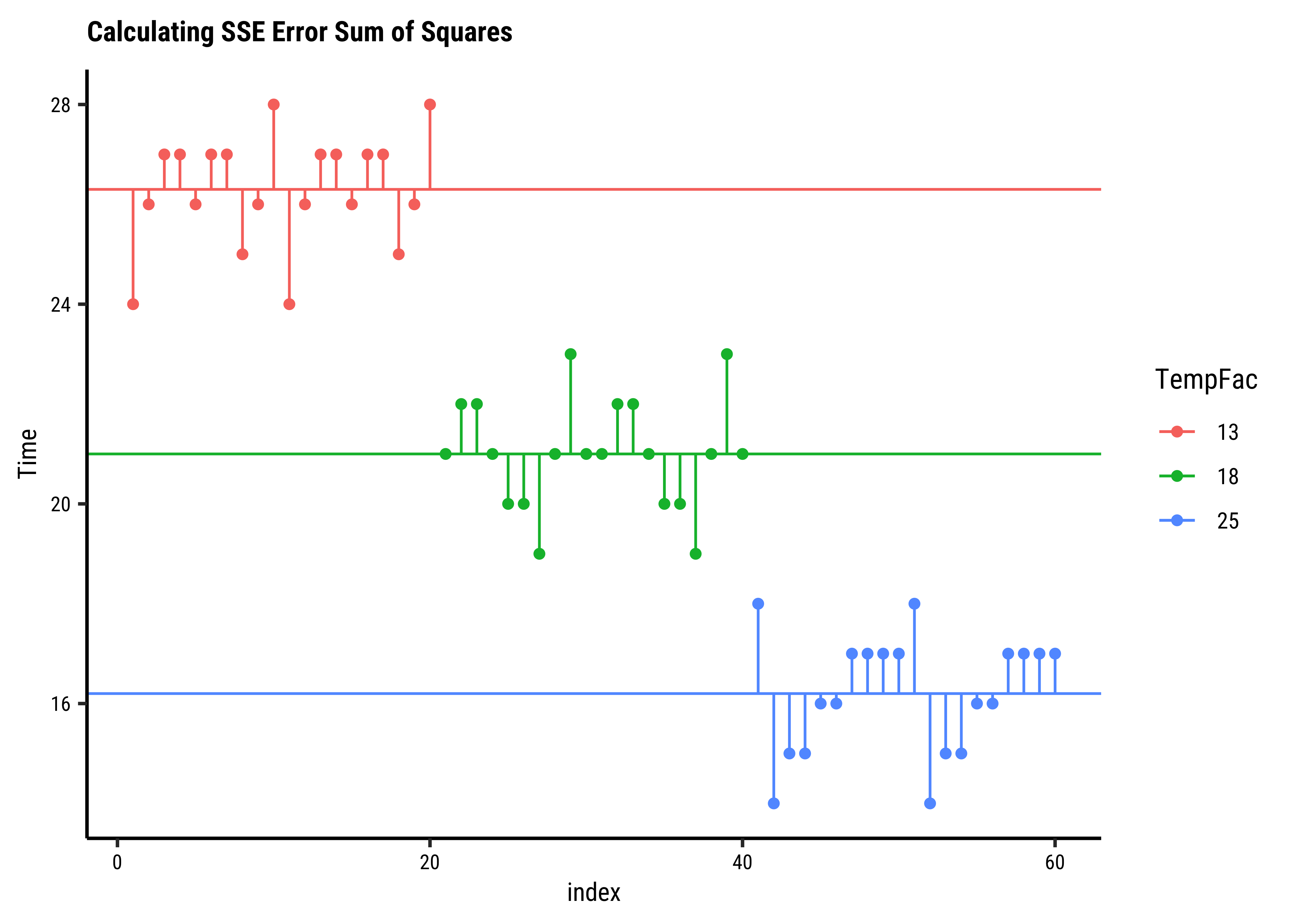
Grouped Data: In Fig B, the horizontal green and red lines are the means of the individual groups, respectively
Improvement: We take the difference in the squared error sums:
Improvement Ratio:
Let us compute these numbers for our toy dataset:
 Analysis of Variance Table (Type III SS)
 Model: quant ~ qual

                               SS df      MS       F   PRE     p
 ----- --------------- | -------- -- ------- ------- ----- -----
 Model (error reduced) |  823.407  1 823.407 139.356 .7857 .0000
 Error (from model)    |  224.529 38   5.909
 ----- --------------- | -------- -- ------- ------- ----- -----
 Total (empty model)   | 1047.935 39  26.870
What do we see?
-
All Data:
-
Grouped Data:
-
Improvement:
-
Improvement Ratio: Before we set up this ratio, we must realize that each of these measures uses a different number of observations! So the comparison is done after scaling each of
-
Large Enough Ratio?: The value of the
F-statisticfrom the table above isF-statisticis compared with a critical value of theF-criticalto help us decide. (Here, it is.) - Belief: So we now believe in the idea of two means.
-
Back to Mean Differences: Finally, in order to find which of the means is significantly different from others (if there are more than two!), we need to make a pair-wise comparison of the means, applying the
Bonferroni correctionas stated before. This means we divide the criticalp.valuewe expect by the number of comparisons we make between levels of the Qual variable.supernovadid this for us in the error-bar plot above.
Why “ANOVA”?
When divide each of
So this may seem like a great Hero’s Journey, where we start with means and differences, go into sums of squares, differences and comparisons of error ratios, and return to the means where we started, only to know them properly now.
Now that we understand what aov() is doing, let us hand-calculate the numbers for our frogs dataset and check. Let us visualize our calculations first.
Let us get the ready table from supernova first, and then systematically calculate all numbers with understanding:
supernova::supernova(frogs_anova) Analysis of Variance Table (Type III SS)
Model: Time ~ TempFac
SS df MS F PRE p
----- --------------- | -------- -- ------- ------- ----- -----
Model (error reduced) | 1020.933 2 510.467 385.897 .9312 .0000
Error (from model) | 75.400 57 1.323
----- --------------- | -------- -- ------- ------- ----- -----
Total (empty model) | 1096.333 59 18.582 Here are the SST, SSE, and the SSA:
# Calculate overall sum squares SST
frogs_overall <- frogs_long %>%
  summarise(
    overall_mean_time = mean(Time),
    # Overall mean across all readings
    # The Black Line

    SST = sum((Time - overall_mean_time)^2),
    n = n()
  ) # Always do this with `summarise`

frogs_overalloverall_mean_time <dbl> | SST <dbl> | n <int> | ||
|---|---|---|---|---|
| 21.16667 | 1096.333 | 60 |
##
SST <- frogs_overall$SST
SST
[1] 1096.333# Calculate sums of square errors *within* each group
# with respect to individual group means
frogs_within_groups <- frogs_long %>%
group_by(TempFac) %>%
summarise(
grouped_mean_time = mean(Time), # The Coloured Lines
grouped_variance_time = var(Time),
group_error_squares = sum((Time - grouped_mean_time)^2),
n = n()
)
frogs_within_groups
##
frogs_SSE <- frogs_within_groups %>%
summarise(SSE = sum(group_error_squares))
##
SSE <- frogs_SSE$SSE
SSETempFac <fct> | grouped_mean_time <dbl> | grouped_variance_time <dbl> | group_error_squares <dbl> | n <int> |
|---|---|---|---|---|
| 13 | 26.3 | 1.273684 | 24.2 | 20 |
| 18 | 21.0 | 1.263158 | 24.0 | 20 |
| 25 | 16.2 | 1.431579 | 27.2 | 20 |
[1] 75.4SST
SSE
SSA <- SST - SSE
SSA[1] 1096.333
[1] 75.4
[1] 1020.933We have
In order to calculate the F-Statistic, we need to compute the variances, using these sum of squares. We obtain variances by dividing by their Degrees of Freedom:
where
Let us calculate these Degrees of Freedom.
With TempFac, and
And therefore
These are, of course, as shown in the df column in the supernova tabel above. We can still calculate these in R, for the sake of method and clarity (and pedantry):
# Error Sum of Squares SSE
df_SSE <- frogs_long %>%
  # Takes into account "unbalanced" situations
  # Where groups are not equal in size
  group_by(TempFac) %>%
  summarise(per_group_df_SSE = n() - 1) %>%
  summarise(df_SSE = sum(per_group_df_SSE)) %>%
  as.numeric()


## Overall Sum of Squares SST
df_SST <- frogs_long %>%
  summarise(df_SST = n() - 1) %>%
  as.integer()


# Treatment Sum of Squares SSA
k <- length(unique(frogs_long$TempFac))
df_SSA <- k - 1
The degrees of freedom for the quantities are:
df_SST
df_SSE
df_SSA
[1] 59
[1] 57
[1] 2Now we are ready to compute the F-statistic: dividing each sum-of-squares byt its degrees of freedom gives us variances which we will compare, using the F-statistic as a ratio:
# Finally F_Stat!
# Combine the sum-square_error for each level of the factor
# Weighted by degrees of freedom **per level**
# Which are of course equal here ;-D

MSE <- frogs_within_groups %>%
  summarise(mean_square_error = sum(group_error_squares / df_SSE)) %>%
  as.numeric()
MSE
[1] 1.322807##
MSA <- SSA / df_SSA # This is OK
MSA[1] 510.4667##
F_stat <- MSA / MSE
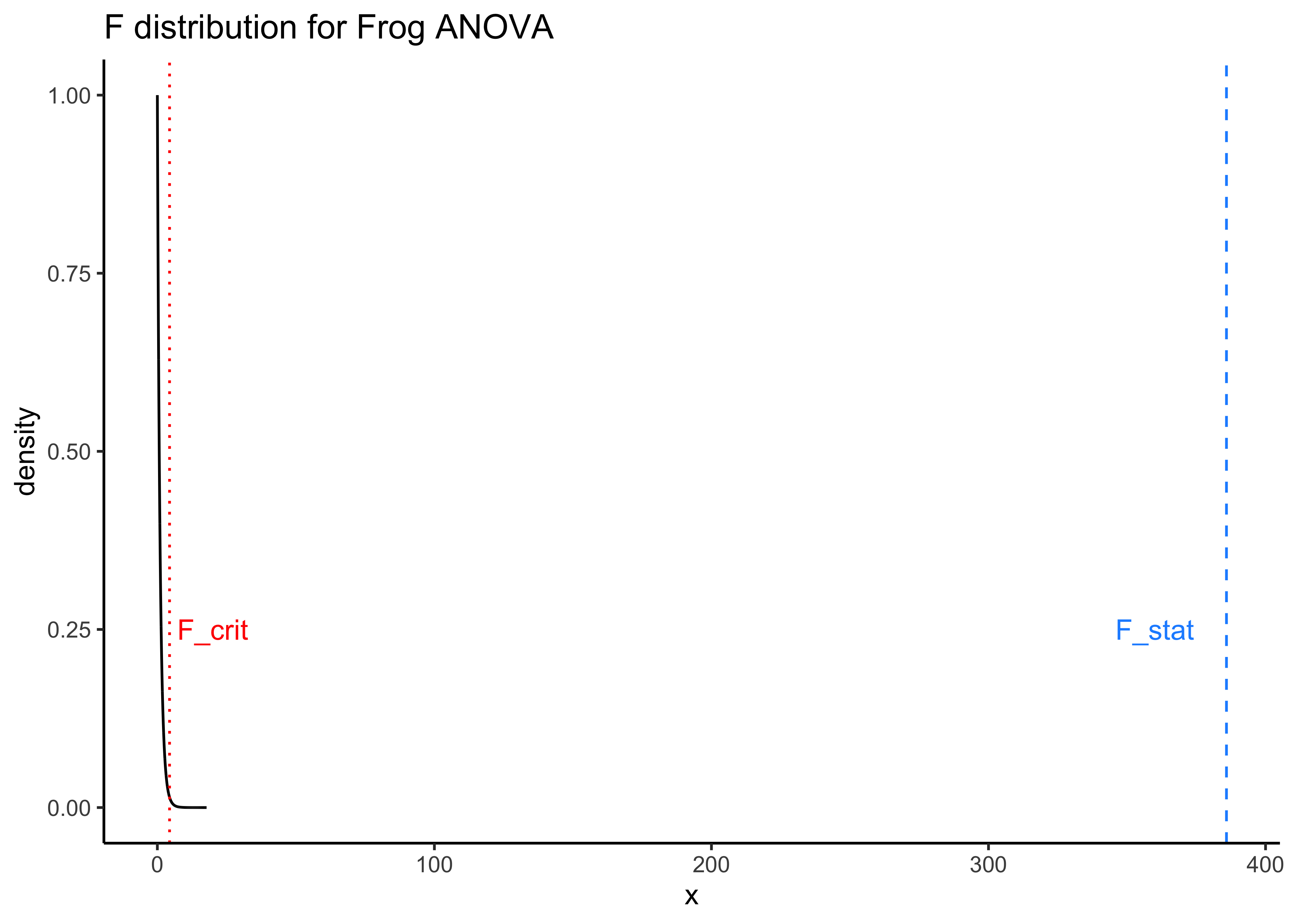
F_stat[1] 385.8966The F-stat is compared with a critical value of the F-statistic, F_crit which is computed using the formula for the f-distribution in R. As with our hypothesis tests, we set the significance level to qf() which computes the critical F value F_critical as a quartile:
F_crit <-
  qf(
    p = (1 - 0.05 / 3), # Significance level is 5% + Bonferroni Correction
    df1 = df_SSA, # Numerator degrees of freedom
    df2 = df_SSE # Denominator degrees of freedom
  )
F_crit
F_stat
[1] 4.403048
[1] 385.8966The F_crit value can also be seen in a plot4,5:
# Set graph theme
theme_set(new = theme_custom())
#
mosaic::xpf(
  q = F_crit,
  df1 = df_SSA, df2 = df_SSE, method = "gg",
  log.p = FALSE, lower.tail = TRUE,
  return = "plot"
) %>%
  gf_vline(xintercept = F_crit) %>%
  gf_label(0.75 ~ 5.5,
    label = "F_critical",
    inherit = F, show.legend = F
  ) %>%
  gf_labs(
    title = "F distribution for Frogs Data",
    subtitle = "F_critical = 4.403"
  )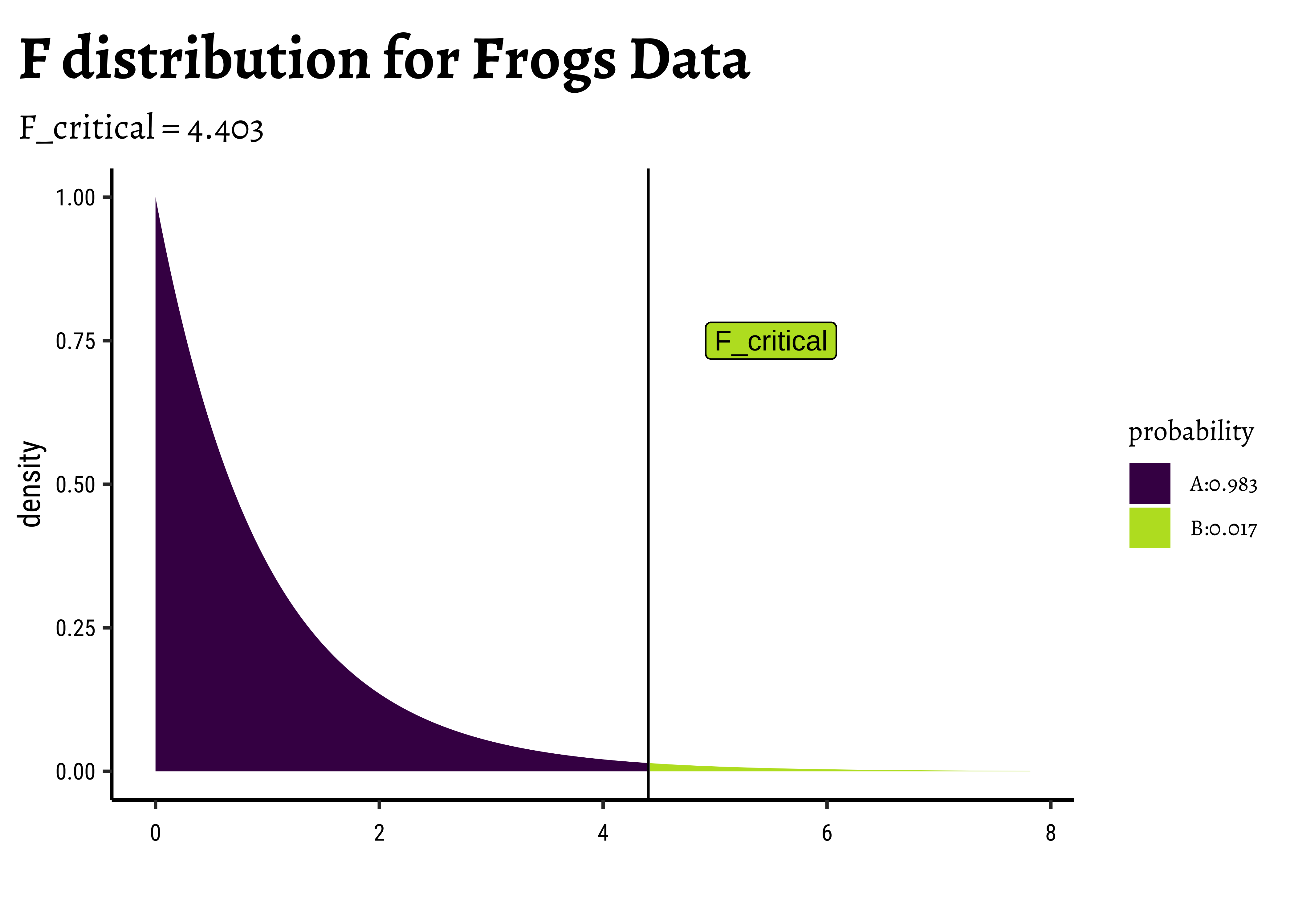
Any value of F more than the F_crit occurs with smaller probability than F_crit, by orders of magnitude! And so we can say with confidence that Temperature has a significant effect on spawn Time.
And that is how ANOVA computes!
And supernova gives us a nice linear equation relating Hatching_Time to TempFac:
supernova::equation(frogs_anova)Fitted equation:
Time = 26.3 + -5.3*TempFac18 + -10.1*TempFac25 + eTempFac18 and TempFac25 are binary {0,1} coded variables, representing the test situation. e is the remaining error. The equation models the means at each value of TempFac.
ANOVA makes 3 fundamental assumptions:
- Data (and errors) are normally distributed.
- Variances are equal.
- Observations are independent.
We can check these using checks and graphs.
The shapiro.wilk test tests if a vector of numeric data is normally distributed and rejects the hypothesis of normality when the p-value is less than or equal to 0.05.
shapiro.test(x = frogs_long$Time)
    Shapiro-Wilk normality test

data:  frogs_long$Time
W = 0.92752, p-value = 0.001561
The p-value is very low and we cannot reject the (alternative) hypothesis that the overall data is not normal. How about normality at each level of the factor?
TempFac <fct> | statistic <dbl> | p.value <dbl> | method <chr> |
|---|---|---|---|
| 13 | 0.8895426 | 0.02637682 | Shapiro-Wilk normality test |
| 18 | 0.9254425 | 0.12614802 | Shapiro-Wilk normality test |
| 25 | 0.8978947 | 0.03766278 | Shapiro-Wilk normality test |
The shapiro.wilk test makes a NULL Hypothesis that the data are normally distributed and estimates the probability that the given data could have happened by chance. Except for TempFac = 18 the p.values are less than 0.05 and we can reject the NULL hypothesis that each of these is normally distributed. Perhaps this is a sign that we need more than 20 samples per factor level. Let there be more frogs !!! இன்னும தவளைகள் வேண்டும்!! !!
We can also check the residuals post-model:
# Set graph theme
theme_set(new = theme_custom())
#
frogs_anova$residuals %>%
  as_tibble() %>%
  gf_dhistogram(~value, data = .) %>%
  gf_labs(
    title = "Residuals Histogram",
    x = "Residuals", y = "Count"
  ) %>%
  gf_fitdistr()
##
frogs_anova$residuals %>%
  as_tibble() %>%
  gf_qq(~value, data = .) %>%
  gf_qqstep() %>%
  gf_labs(
    title = "Residuals Q-Q Plot",
    x = "Theoretical Quantiles", y = "Sample Quantiles"
  ) %>%
  gf_qqline()
##
shapiro.test(frogs_anova$residuals)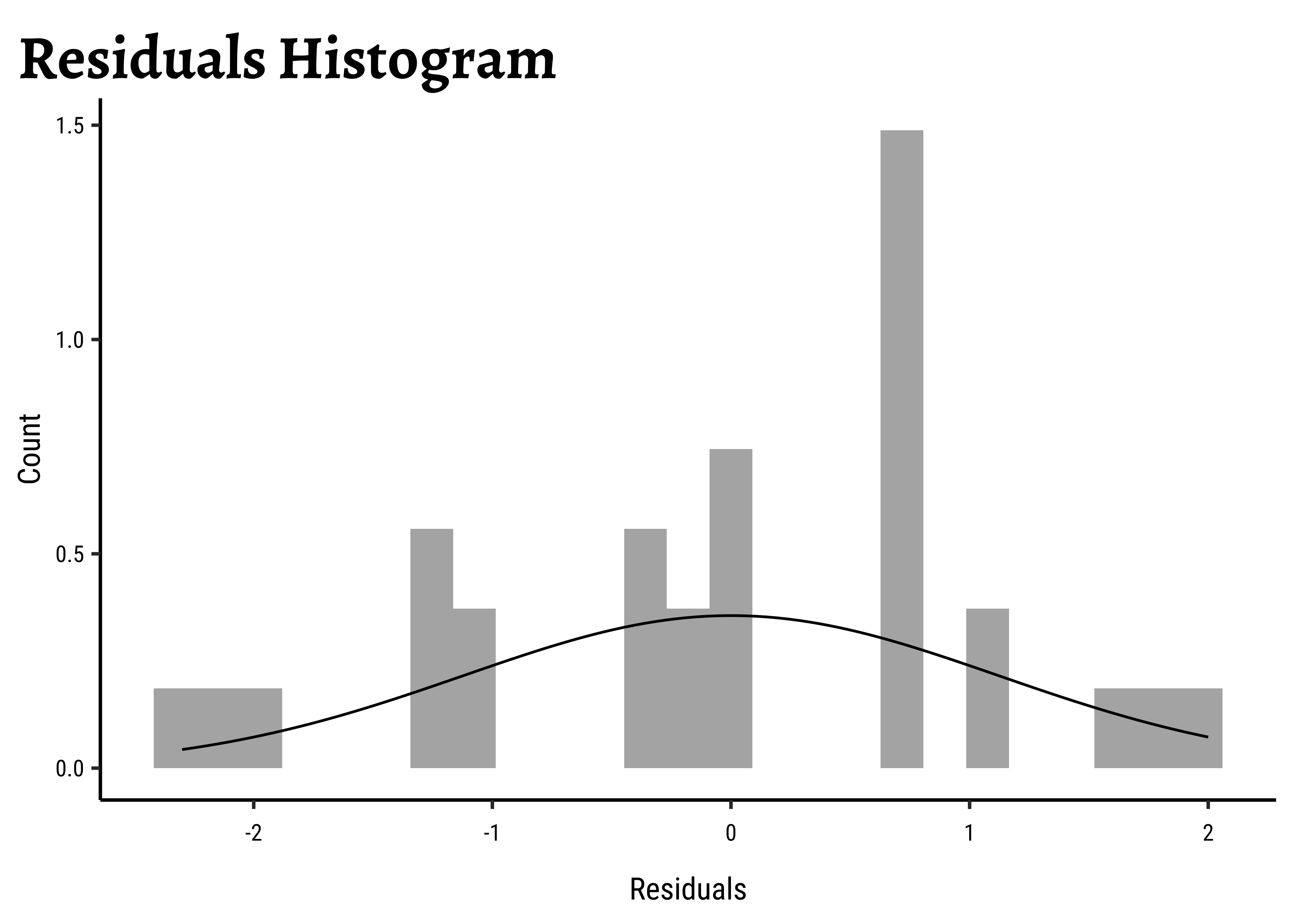
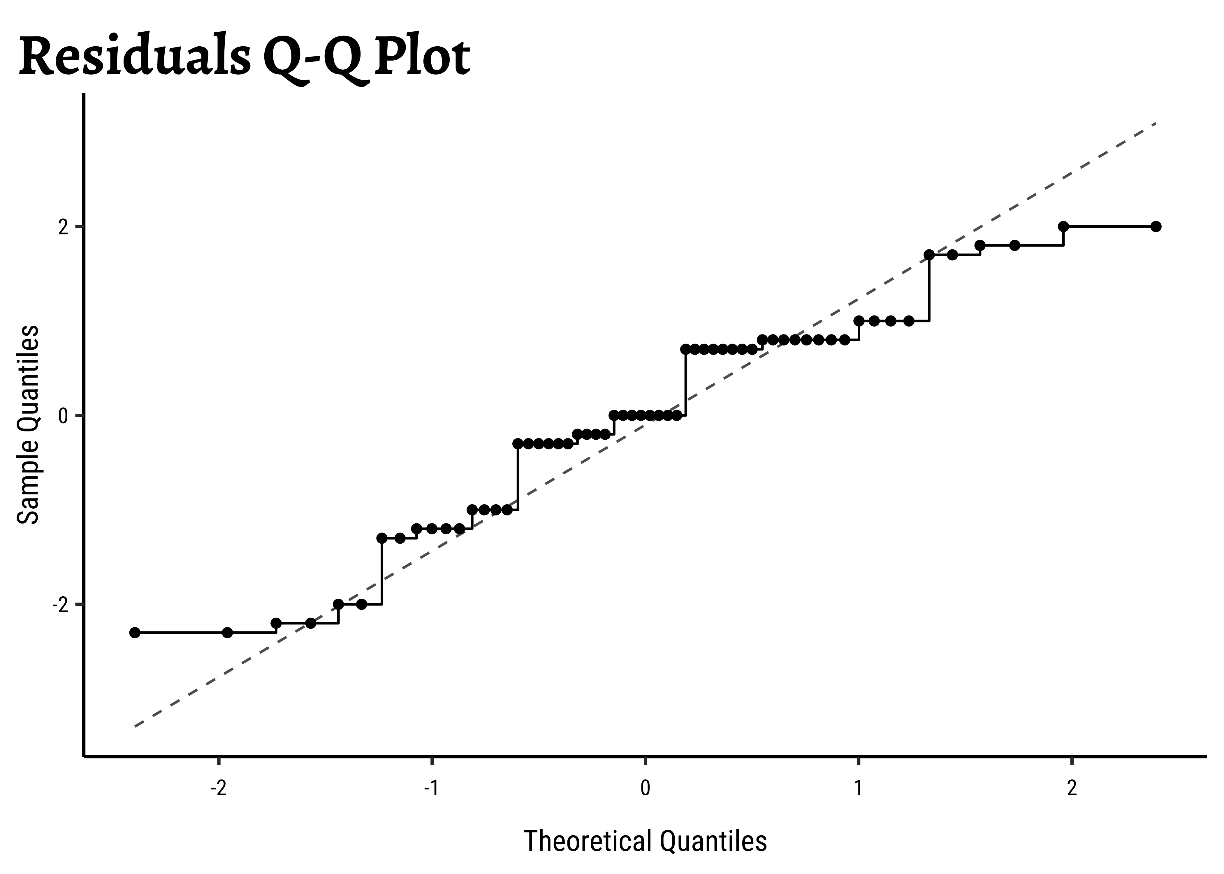
    Shapiro-Wilk normality test

data:  frogs_anova$residuals
W = 0.94814, p-value = 0.01275
Unsurprisingly, the residuals are also not normally distributed either.
Response data with different variances at different levels of an explanatory variable are said to exhibit heteroscedasticity. This violates one of the assumptions of ANOVA.
To check if the Time readings are similar in variance across levels of TempFac, we can use the Levene Test, or since our per-group observations are not normally distributed, a non-parametric rank-based Fligner-Killeen Test. The NULL hypothesis is that the data are with similar variances. The tests assess how probable this is with the given data assuming this NULL hypothesis:
frogs_long %>%
  group_by(TempFac) %>%
  summarise(variance = var(Time))
# Not too different...OK on with the test
DescTools::LeveneTest(Time ~ TempFac, data = frogs_long)
##
fligner.test(Time ~ TempFac, data = frogs_long)TempFac <fct> | variance <dbl> | |||
|---|---|---|---|---|
| 13 | 1.273684 | |||
| 18 | 1.263158 | |||
| 25 | 1.431579 |
Df <int> | F value <dbl> | Pr(>F) <dbl> | ||
|---|---|---|---|---|
| group | 2 | 0.3931034 | 0.6767746 | |
| 57 | NA | NA |
    Fligner-Killeen test of homogeneity of variances

data:  Time by TempFac
Fligner-Killeen:med chi-squared = 0.53898, df = 2, p-value = 0.7638
It seems that there is no cause for concern here; the data do not have significantly different variances.
This is an experiment design concern; the way the data is gathered must be specified such that data for each level of the factors ( factor combinations if there are more than one) should be independent.
The simplest way to find the actual effect sizes detected by an ANOVA test is something we have already done, with the supernova package: Here is the table and plot again:
# Set graph theme
theme_set(new = theme_custom())
#
frogs_supernova <-
  supernova::pairwise(frogs_anova,
    plot = TRUE,
    alpha = 0.05,
    correction = "Bonferroni"
  )
frogs_supernova
  group_1 group_2    diff pooled_se       t    df   lower  upper p_adj
  <chr>   <chr>     <dbl>     <dbl>   <dbl> <int>   <dbl>  <dbl> <dbl>
1 18      13       -5.300     0.257 -20.608    57  -5.861 -4.739 .0000
2 25      13      -10.100     0.257 -39.272    57 -10.661 -9.539 .0000
3 25      18       -4.800     0.257 -18.664    57  -5.361 -4.239 .0000
This table, the plot, and the equation we set up earlier all give us the sense of how the TempFac affects Time. The differences are given pair-wise between levels of the Qual factor, TempFac, and the standard error has been declared in pooled fashion (all groups together).
We can also use (paradoxically) the summary.lm() command:
tidy_anova <-
  frogs_anova %>%
  summary.lm() %>%
  broom::tidy()
tidy_anovaterm <chr> | estimate <dbl> | std.error <dbl> | statistic <dbl> | p.value <dbl> |
|---|---|---|---|---|
| (Intercept) | 26.3 | 0.2571777 | 102.26394 | 2.781059e-66 |
| TempFac18 | -5.3 | 0.3637041 | -14.57228 | 7.081214e-21 |
| TempFac25 | -10.1 | 0.3637041 | -27.76982 | 8.187867e-35 |
It may take a bit of effort to understand this. First the TempFac is arranged in order of levels, and the mean at the Intercept. That is p.value for all these effect sizes is well below the desired confidence level of
Standard Errors
Observe that the std.error for the intercept is TempFac18 and TempFac25 is
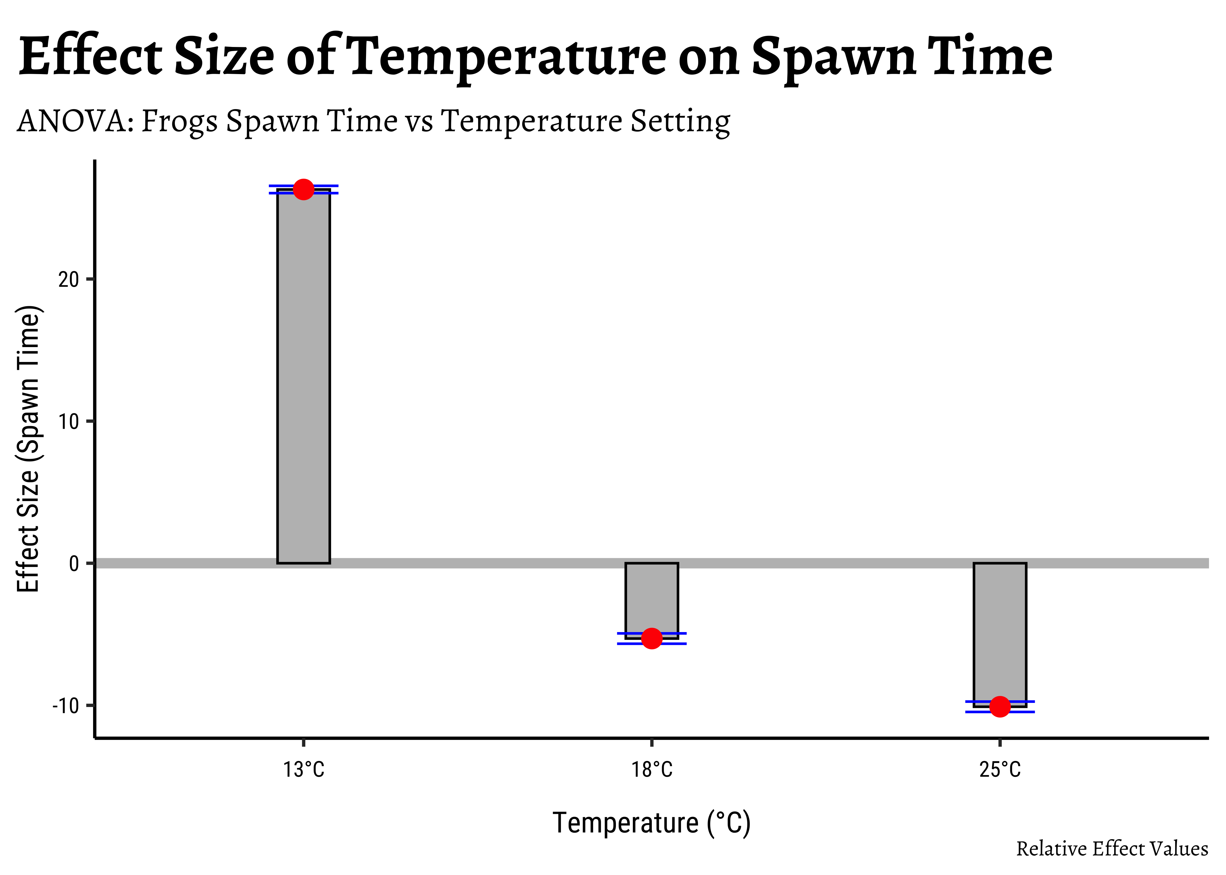
We can easily plot bar-chart with error bars for the effect size:
# Set graph theme
theme_set(new = theme_custom())
#
tidy_anova %>%
  mutate(
    hi = estimate + std.error,
    lo = estimate - std.error
  ) %>%
  gf_hline(
    data = ., yintercept = 0,
    colour = "grey",
    linewidth = 2
  ) %>%
  gf_col(estimate ~ term,
    fill = "grey",
    color = "black",
    width = 0.15
  ) %>%
  gf_errorbar(hi + lo ~ term,
    color = "blue",
    width = 0.2
  ) %>%
  gf_point(estimate ~ term,
    color = "red",
    size = 3.5
  ) %>%
  gf_refine(scale_x_discrete("Temperature (°C)",
    labels = c("13°C", "18°C", "25°C")
  )) %>%
  gf_labs(
    title = "Effect Size of Temperature on Spawn Time",
    subtitle = "ANOVA: Frogs Spawn Time vs Temperature Setting",
    caption = "Relative Effect Values",
    x = "Temperature (°C)", y = "Effect Size (Spawn Time)"
  )
If we want an “absolute value” plot for effect size, it needs just a little bit of work:
# Merging group averages with `std.error`
# Set graph theme
theme_set(new = theme_custom())
#

frogs_long %>%
  group_by(TempFac) %>%
  summarise(mean = mean(Time)) %>%
  cbind(std.error = tidy_anova$std.error) %>%
  mutate(
    hi = mean + std.error,
    lo = mean - std.error
  ) %>%
  gf_hline(
    data = ., yintercept = 0,
    colour = "grey",
    linewidth = 2
  ) %>%
  gf_col(mean ~ TempFac,
    fill = "grey",
    color = "black", width = 0.15
  ) %>%
  gf_errorbar(hi + lo ~ TempFac,
    color = "blue",
    width = 0.2
  ) %>%
  gf_point(mean ~ TempFac,
    color = "red",
    size = 3.5
  ) %>%
  gf_refine(scale_x_discrete("Temperature (°C)",
    labels = c("13°C", "18°C", "25°C")
  )) %>%
  gf_labs(
    title = "Effect Size of Temperature on Spawn Time",
    subtitle = "ANOVA: Frogs Spawn Time vs Temperature Setting",
    caption = "Absolute Effect Values",
    x = "Temperature (°C)", y = "Effect Size (Spawn Time)"
  )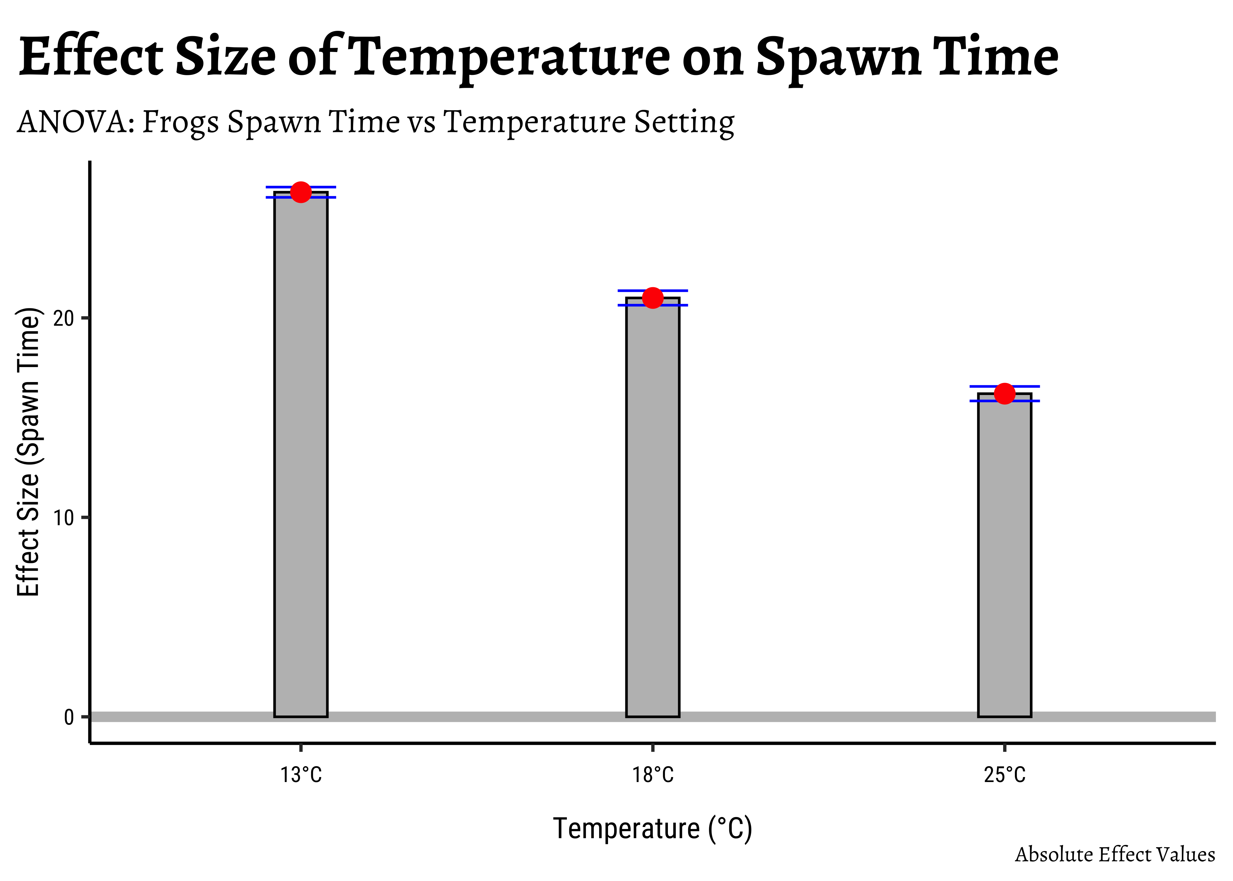
In both graphs, note the difference in the error-bar heights.
The ANOVA test does not tell us that the “treatments” (i.e. levels of TempFac) are equally effective. We need to use a multiple comparison procedure to arrive at an answer to that question. We compute the pair-wise differences in effect-size:
  Tukey multiple comparisons of means
    95% family-wise confidence level

Fit: aov(formula = Time ~ TempFac, data = frogs_long)

$TempFac
       diff        lwr       upr p adj
18-13  -5.3  -6.175224 -4.424776     0
25-13 -10.1 -10.975224 -9.224776     0
25-18  -4.8  -5.675224 -3.924776     0
We see that each of the pairwise differences in effect-size is significant, with p = 0 !
We wish to establish the significance of the effect size due to each of the levels in TempFac. From the normality tests conducted earlier we see that except at one level of TempFac, the times are are not normally distributed. Hence we opt for a Permutation Test to check for significance of effect.
As remarked in Ernst8, the non-parametric permutation test can be both exact and also intuitively easier for students to grasp.
We proceed with a Permutation Test for TempFac. We shuffle the levels (13, 18, 25) randomly between the Times and repeat the ANOVA test each time and calculate the F-statistic. The Null distribution is the distribution of the F-statistic over the many permutations and the p-value is given by the proportion of times the F-statistic equals or exceeds that observed.
We will use infer to do this: We calculate the observed F-stat with infer, which also has a very direct, if verbose, syntax for doing permutation tests:
observed_infer <-
  frogs_long %>%
  specify(Time ~ TempFac) %>%
  hypothesise(null = "independence") %>%
  calculate(stat = "F")
observed_inferstat <dbl> | ||||
|---|---|---|---|---|
| 385.8966 |
We see that the observed F-Statistic is of course infer to generate a NULL distribution using permutation of the factor TempFac:
null_dist_infer <- frogs_long %>%
  specify(Time ~ TempFac) %>%
  hypothesise(null = "independence") %>%
  generate(reps = 4999, type = "permute") %>%
  calculate(stat = "F")
##
null_dist_inferreplicate <int> | stat <dbl> | |||
|---|---|---|---|---|
| 1 | 1.9359049289 | |||
| 2 | 2.9119835126 | |||
| 3 | 0.3322413952 | |||
| 4 | 0.1998254799 | |||
| 5 | 1.9329404889 | |||
| 6 | 1.0130820818 | |||
| 7 | 1.0409851565 | |||
| 8 | 0.9629891561 | |||
| 9 | 2.4882971338 | |||
| 10 | 0.1366969114 |
##
null_dist_infer %>%
  visualise(method = "simulation") +
  shade_p_value(obs_stat = observed_infer$stat, direction = "right") +
  scale_x_continuous(trans = "log10", expand = c(0, 0)) +
  coord_cartesian(xlim = c(0.2, 500), clip = "off") +
  annotation_logticks(outside = FALSE) +
  theme_custom()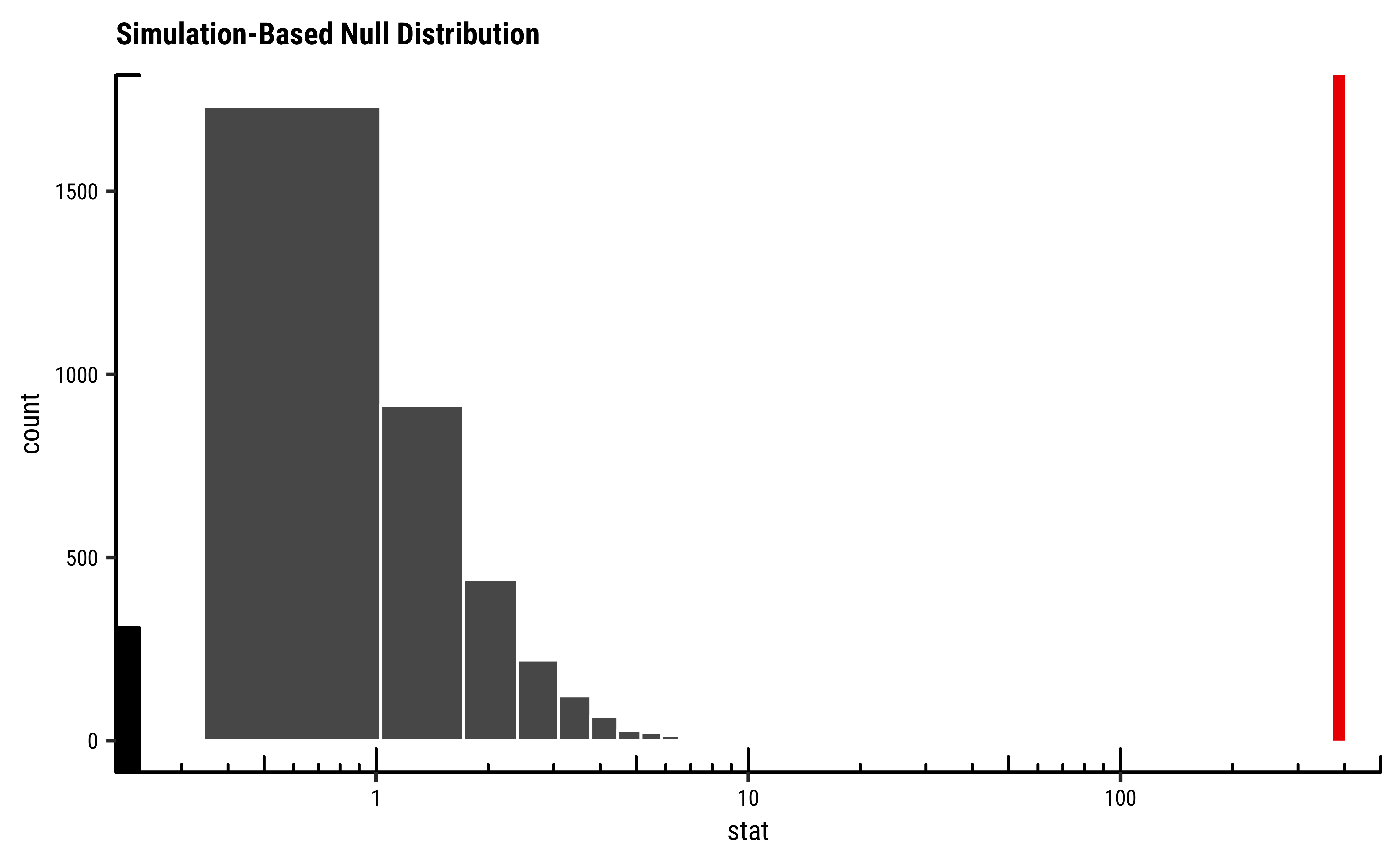
As seen, the infer based permutation test also shows that the permutationally generated F-statistics are nowhere near that which was observed. The effect of TempFac is very strong.
- In marketing, design, or business research, similar quantities may be measured across different locations, or stores, or categories of people, for instance.
- ANOVA is the tool to decide if the Quant variable has differences across the Qual categories.
- This approach can be extended to more than one Qual variable, and also if there is another Quant variable in the mix.
We have discussed ANOVA as a means of modelling the effects of a Categorical variable on a Continuous (Quant) variable. ANOVA can be carried out using the standard formula aov when assumptions on distributions, variances, and independence are met. Permutation ANOVA tests can be carried out when these assumptions do not quite hold.
Two-Way ANOVA
What if we have two Categorical variables as predictors?
We then need to perform a Two-Way ANOVA analysis, where we look at the predictors individually (main effects) and together (interaction effects). Here too, we need to verify if the number of observations are balanced across all combinations of factors of the two Qualitative predictors. There are three different classical approaches (Type1, Type2, and Type3 ANOVA) for testing hypotheses in ANOVA for unbalanced designs, as they are called. (Langsrud 2003).
Informative Hypothesis Testing: Models which incorporate a priori Beliefs
Note that when we specified our research question, we had no specific hypothesis about the means, other than that they might be different. In many situations, we may have reason to believe in the relative “ordering” of the means for different levels of the Categorical variable. The one-sided t-test is the simplest example (e.g.,
It is possible to incorporate these beliefs into the ANOVA model, using what is called as informative hypothesis testing, which have certain advantages compared to unconstrained models. The R package called restriktor has the capability to develop such models with beliefs.
Try the simple datasets at https://www.performingmusicresearch.com/datasets/
Can you try to ANOVA-analyse the datasets we dealt with in plotting Groups with Boxplots?
- The ANOVA tutorial at Our Coding Club
- Antoine Soetewey. How to: one-way ANOVA by hand. https://statsandr.com/blog/how-to-one-way-anova-by-hand/
- ANOVA in R - Stats and R https://statsandr.com/blog/anova-in-r/
- Michael Crawley.(2013) The R Book,second edition. Chapter 11.
- David C Howell, Permutation Tests for Factorial ANOVA Designs
- Marti Anderson, Permutation tests for univariate or multivariate analysis of variance and regression
- Judd, Charles M., Gary H. McClelland, and Carey S. Ryan.(2017). “Introduction to Data Analysis.” In, 1–9. Routledge. https://doi.org/10.4324/9781315744131-1.
- Patil, I. (2021). Visualizations with statistical details: The ‘ggstatsplot’ approach. Journal of Open Source Software, 6(61), 3167, doi:10.21105/joss.03167
- Langsrud, Øyvind. (2003). ANOVA for unbalanced data: Use type II instead of type III sums of squares. Statistics and Computing. 13. 163-167. https://doi.org/10.1023/A:1023260610025. https://www.researchgate.net/publication/220286726_ANOVA_for_unbalanced_data_Use_type_II_instead_of_type_III_sums_of_squares
- Kim TK. (2017). Understanding one-way ANOVA using conceptual figures. Korean J Anesthesiol. 2017 Feb;70(1):22-26. https://ekja.org/upload/pdf/kjae-70-22.pdf
- Anova – Type I/II/III SS explained.https://mcfromnz.wordpress.com/2011/03/02/anova-type-iiiiii-ss-explained/
- Bidyut Ghosh (Aug 28, 2017). One-way ANOVA in R. https://datascienceplus.com/one-way-anova-in-r/
Blake, Adam, Jeff Chrabaszcz, Ji Son, and Jim Stigler. 2024. supernova: Judd, McClelland, & Ryan Formatting for ANOVA Output. https://doi.org/10.32614/CRAN.package.supernova.
Dawson, Charlotte. 2025. ggprism: A “ggplot2” Extension Inspired by “GraphPad Prism”. https://doi.org/10.32614/CRAN.package.ggprism.
Langsrud, Øyvind. 2003. Statistics and Computing 13 (2): 163–67. https://doi.org/10.1023/a:1023260610025.
Patil, Indrajeet. 2021. “Visualizations with statistical details: The ‘ggstatsplot’ approach.” Journal of Open Source Software 6 (61): 3167. https://doi.org/10.21105/joss.03167.
Signorell, Andri. 2025. DescTools: Tools for Descriptive Statistics. https://doi.org/10.32614/CRAN.package.DescTools.
Vanbrabant, Leonard, and Rebecca Kuiper. 2024. restriktor: Restricted Statistical Estimation and Inference for Linear Models. https://doi.org/10.32614/CRAN.package.restriktor.
Wilke, Claus O., and Brenton M. Wiernik. 2022. ggtext: Improved Text Rendering Support for “ggplot2”. https://doi.org/10.32614/CRAN.package.ggtext.
Footnotes
The ANOVA tutorial at Our Coding Club.↩︎
Pruim R, Kaplan DT, Horton NJ (2017). “The mosaic Package: Helping Students to ‘Think with Data’ Using R.” The R Journal, 9(1), 77–102. https://journal.r-project.org/archive/2017/RJ-2017-024/index.html.↩︎
mosaic::xpf()gives both a graph and the probabilities.↩︎ggplot2 Based Plots with Statistical Details • ggstatsplot https://indrajeetpatil.github.io/ggstatsplot/↩︎
Ernst, Michael D. 2004. “Permutation Methods: A Basis for Exact Inference.” Statistical Science 19 (4): 676–85. doi:10.1214/088342304000000396.↩︎
Citation
BibTeX citation:
@online{2023,
  author = {},
  title = {Comparing {Multiple} {Means} with {ANOVA}},
  date = {2023-03-28},
  url = {https://av-quarto.netlify.app/content/courses/Analytics/Inference/Modules/130-ThreeMeansOrMore/},
  langid = {en},
  abstract = {ANOVA to investigate how frogspawn hatching time varies
    with temperature.}
}
For attribution, please cite this work as:
“Comparing Multiple Means with ANOVA.” 2023. March 28,
2023. https://av-quarto.netlify.app/content/courses/Analytics/Inference/Modules/130-ThreeMeansOrMore/.