🃏 Testing a Single Proportion

Abstract

Inference Tests for the significance of a Proportion

Setting up R packages

library(tidyverse)
library(mosaic)
library(ggformula)
library(infer)

## Datasets from Chihara and Hesterberg's book (Second Edition)
library(resampledata)

## Datasets from Cetinkaya-Rundel and Hardin's book (First Edition)
library(openintro)

Introduction

Often we hear reports that a certain percentage of people support a certain political party, or that a certain proportion of people are in favour of a certain policy. Such statements are the result of a desire to infer a proportion in the population, which is what we will investigate here.

Workflow: Sampling Theory for Proportions

We have seen how sampling from a population works when we wish to estimate means:

• The sample means $\overline{x}$ are centred around the population mean $\mu$;
• The samples means are normally distributed
• The uncertainty in using $\overline{x}$ as an estimate for $\mu$ is given by a Confidence interval defined by some constant times the Standard Error of the sample $\frac{s}{\sqrt{(}n)}$;
• The larger the size of the sample, the tighter the Confidence Interval.

Now then: does a similar logic work for proportions too, as for means?

The CLT for Proportions

• Sample proportions are also centred around population proportions
• Success-failure condition: If $\hat{p}\ast n>=10$ and $(1-\hat{p})\ast n>=10$ are both satisfied, then the we can assume that the sampling distribution of the proportion is normal. And so:
• The Standard Error for a sample proportion is given by $SE=\sqrt{\frac{\hat{p}(1-\hat{p})}{n}}$, where $\hat{p}$ is the sample proportion
• We would calculate the Confidence Intervals in a similar fashion, based on the desired probability of error, as:

$$p=\hat{p}\pm 1.96\ast SE$$

Case Study #1: YRBSS Survey

We will be analyzing the same dataset called the Youth Risk Behavior Surveillance System (YRBSS) survey from the openintro package, which uses data from high schoolers to help discover health patterns. The dataset is called yrbss.

Workflow: Read the Data

data(yrbss, package = "openintro")
yrbss

ABCDEFGHIJ0123456789

age <int>	gender <chr>	grade <chr>	hispanic <chr>	race <chr>	height <dbl>	weight <dbl>	helmet_12m <chr>
14	female	9	not	Black or African American	NA	NA	never
14	female	9	not	Black or African American	NA	NA	never
15	female	9	hispanic	Native Hawaiian or Other Pacific Islander	1.73	84.37	never
15	female	9	not	Black or African American	1.60	55.79	never
15	female	9	not	Black or African American	1.50	46.72	did not ride
15	female	9	not	Black or African American	1.57	67.13	did not ride
15	female	9	not	Black or African American	1.65	131.54	did not ride
14	male	9	not	Black or African American	1.88	71.22	never
15	male	9	not	Black or African American	1.75	63.50	never
15	male	10	not	Black or African American	1.37	97.07	did not ride

Next

123456

...

1000

Previous

1-10 of 10,000 rows | 1-8 of 13 columns

When summarizing the YRBSS data, the Centers for Disease Control and Prevention seeks insight into the population parameters. Accordingly, in this tutorial, our research questions are:

NoteResearch Questions

1. What are the counts within each category for the amount of days these students have texted while driving within the past 30 days?

2. What proportion of people on earth have texted while driving each day for the past 30 days without wearing helmets?

Question 1 pertains to the data set yrbss, our “sample”. To answer this, you can answer the question, “What proportion of people in your sample reported that they have texted while driving each day for the past 30 days?” with a statistic. Question 2 is an inference we need to make about the population of highschoolers. While the question “What proportion of people on earth have texted while driving each day for the past 30 days?” is answered with an estimate of the parameter.

For our first Research Question, we will choose the column helmet_12m: Remember that you can use filter to limit the dataset to just non-helmet wearers. Here, we will name the (filtered ) dataset no_helmet.

yrbss %>%
  group_by(helmet_12m) %>%
  count()

ABCDEFGHIJ0123456789

helmet_12m <chr>	n <int>
always	399
did not ride	4549
most of time	293
never	6977
rarely	713
sometimes	341
NA	311

7 rows

##
yrbss %>%
  group_by(text_while_driving_30d) %>%
  count()

ABCDEFGHIJ0123456789

text_while_driving_30d <chr>	n <int>
0	4792
1-2	925
10-19	373
20-29	298
3-5	493
30	827
6-9	311
did not drive	4646
NA	918

9 rows

Also, it may be easier to calculate the proportion if we create a new variable that specifies whether the individual has texted every day while driving over the past 30 days or not. We will call this variable text_ind.

no_helmet_text <- yrbss %>%
  filter(helmet_12m == "never") %>%
  mutate(text_ind = ifelse(text_while_driving_30d == "30", "yes", "no")) %>%
  # removing most of the other variables
  select(age, gender, text_ind)
no_helmet_text

ABCDEFGHIJ0123456789

age <int>	gender <chr>	text_ind <chr>
14	female	no
14	female	NA
15	female	yes
15	female	no
14	male	NA
15	male	NA
16	male	no
14	male	no
15	male	no
16	male	no

Next

123456

...

698

Previous

1-10 of 6,977 rows

##
no_helmet_text %>%
  drop_na() %>%
  count(text_ind)

ABCDEFGHIJ0123456789

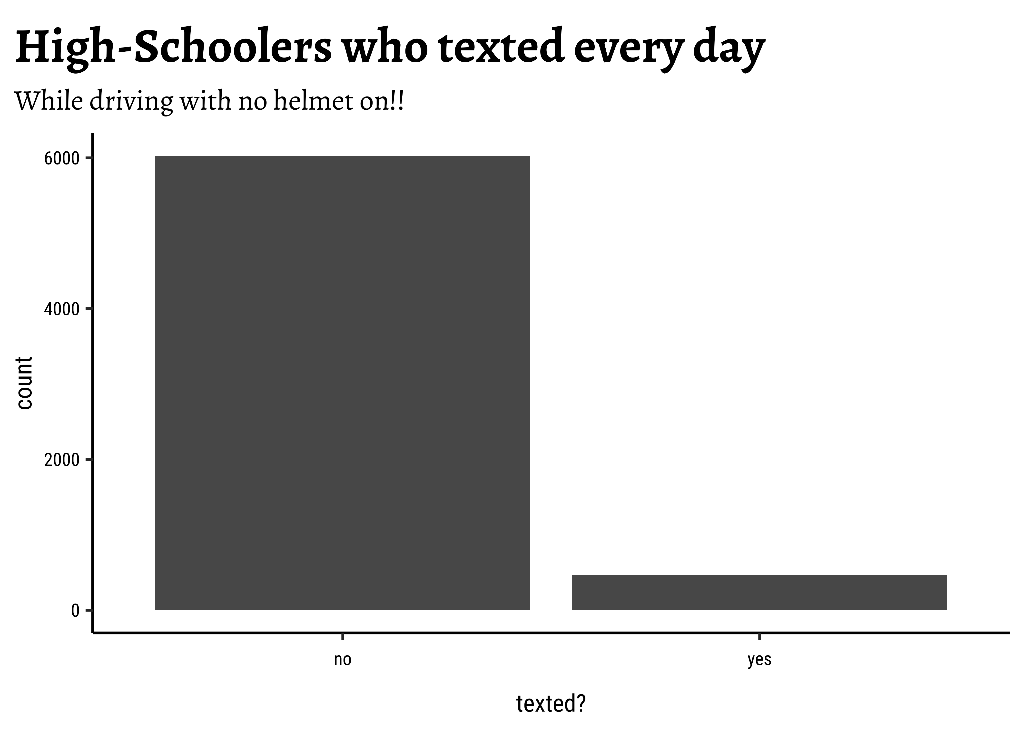
text_ind <chr>	n <int>
no	6025
yes	462

2 rows

##
no_helmet_text %>%
  drop_na() %>%
  summarize(prop = prop(text_ind, success = "yes"), n = n())

ABCDEFGHIJ0123456789

prop <dbl>	n <int>
0.07121936	6487

1 row

This is the observed_statistic: the proportion of people in this sample who do text when they drive without a helmet.

Visualizing a Single Proportion

We can quickly plot this, just for the sake of visual understanding of the proportions:

# Set graph theme
theme_set(new = theme_custom())
#
no_helmet_text %>%
  drop_na() %>%
  gf_bar(~text_ind) %>%
  gf_labs(
    x = "texted?",
    title = "High-Schoolers who texted every day",
    subtitle = "While driving with no helmet on!!"
  )

Inference for a Single Proportion

Based on this sample in the yrbss data, we wish to infer proportions for the population of high-schoolers.

Hypothesis Testing for a Single Proportion

Consider the inference we did for a single mean. What was our NULL Hypothesis? That the population mean $\mu =0$. for two means? That they might be equal. What might a suitable NULL Hypothesis be for a single proportion? What attitude of ain’t nothing happenin’ might we adopt?

Important

With proportions, we usually look for a “no difference” situation, i.e. a ratio of unity!! So our NULL hypothesis would be a proportion of 1:1 for texters and no-texters, so a proportion of $0.5$!!

Classical Test

The simplest test in R for a single proportion is the binom.test:

mosaic::binom.test(~text_ind, data = no_helmet_text, success = "yes")

data:  no_helmet_text$text_ind  [with success = yes]
number of successes = 463, number of trials = 6503, p-value < 2.2e-16
alternative hypothesis: true probability of success is not equal to 0.5
95 percent confidence interval:
 0.06506429 0.07771932
sample estimates:
probability of success 
            0.07119791 

mosaic::binom.test(~text_ind, data = no_helmet_text, success = "yes") %>%
  broom::tidy()

ABCDEFGHIJ0123456789

estimate <dbl>	statistic <dbl>	p.value <dbl>	parameter <dbl>	conf.low <dbl>	conf.high <dbl>	alternative <chr>
0.07119791	463	0	6503	0.06506429	0.07771932	two.sided

1 row

How do we understand this result? That the sample tells us the $\hat{p}=0.07119$ and that based on this the population proportion of those who text while driving without a helmet is also not 0.5, since the p-value is $2.2e-16$. So we reject the NULL hypothesis and accept the alternative hypothesis.

Uncertainty in Estimation

The Confidence Intervals from the binom.test inform us about our population proportion estimate: It lies within the interval [0.06506429, 0.07771932]. We know that this is also given by:

$$ $$\begin{array}{rcl}CI& =& \hat{p}\pm 1.96\ast SE\\ & =& \hat{p}\pm 1.96\ast \sqrt{\hat{p}\ast (1-\hat{p})/n}\\ & =& 0.0711\pm 1.96\ast \sqrt{0.0711\ast (1-0.0711)/6847}\\ & =& 0.0711\pm 0.006\\ & =& [0.065,0.771]\end{array}$$ $$

Permutation Visually Demonstrated

We saw from the diagram created by Allen Downey that there is only one test! We will now use this philosophy to develop a technique that allows us to mechanize several Statistical Models in that way, with nearly identical code. We will first look visually at a permutation exercise. We will create dummy data that contains the following case study:

A set of identical resumes was sent to male and female evaluators. The candidates in the resumes were of both genders. We wish to see if there was difference in the way resumes were evaluated, by male and female evaluators. (We use just one male and one female evaluator here, to keep things simple!)

ABCDEFGHIJ0123456789

evaluator <fct>	candidate_selected <dbl>
F	1
F	1
F	1
F	1
F	1
F	1
F	1
F	1
F	0
F	1

Next

12345

Previous

1-10 of 48 rows

ABCDEFGHIJ0123456789

evaluator <fct>	selection_ratio <dbl>	count <int>	n <int>
F	0.1250000	3	24
M	0.4583333	11	24

2 rows

         M 
-0.3333333 

So, we have a solid disparity in percentage of selection between the two evaluators! Now we pretend that there is no difference between the selections made by either set of evaluators. So we can just:

• Pool up all the evaluations
  
• Arbitrarily re-assign a given candidate(selected or rejected) to either of the two sets of evaluators, by permutation.
  

How would that pooled shuffled set of evaluations look like?

ABCDEFGHIJ0123456789

evaluator <fct>	selection_ratio <dbl>	count <int>	n <int>
F	0.2500000	6	24
M	0.3333333	8	24

2 rows

 

As can be seen, the ratio is different!

We can now check out our Hypothesis that there is no bias. We can shuffle the data many many times, calculating the ratio each time, and plot the distribution of the differences in selection ratio and see how that artificially created distribution compares with the originally observed figure from Mother Nature.

# Set graph theme
theme_set(new = theme_custom())
#
null_dist <- do(4999) * diff(mean(
  candidate_selected ~ shuffle(evaluator),
  data = data
))
# null_dist %>% names()
null_dist %>%
  gf_histogram(~M,
    fill = ~ (M <= obs_difference),
    bins = 25, show.legend = FALSE,
    xlab = "Bias Proportion",
    ylab = "How Often?",
    title = "Permutation Test on Difference between Groups",
    subtitle = ""
  ) %>%
  gf_vline(xintercept = ~obs_difference, color = "red") %>%
  gf_label(500 ~ obs_difference,
    label = "Observed\n Bias",
    show.legend = FALSE
  )
mean(~ M <= obs_difference, data = null_dist)

 

[1] 0.00220044

We see that the artificial data can hardly ever ($p=0.0022$) mimic what the real world experiment is showing. Hence we had good reason to reject our NULL Hypothesis that there is no bias.

Bootstrap test

The inferential tools for estimating a single population proportion are analogous to those used for estimating single population means: the bootstrap confidence interval and the hypothesis test.

no_helmet_text %>%
  drop_na() %>%
  specify(response = text_ind, success = "yes") %>%
  generate(reps = 999, type = "bootstrap") %>%
  calculate(stat = "prop") %>%
  get_ci(level = 0.95)

ABCDEFGHIJ0123456789

lower_ci <dbl>	upper_ci <dbl>
0.06474487	0.07739325

1 row

Note that since the goal is to construct an interval estimate for a proportion, it’s necessary to both include the success argument within specify, which accounts for the proportion of non-helmet wearers than have consistently texted while driving the past 30 days, in this example, and that stat within calculate is here “prop”, signaling that we are trying to do some sort of inference on a proportion.

Case Study #2: TBD

To be Written up in the foreseeable future.

An interactive app

https://openintro.shinyapps.io/CLT_prop/

Wait, But Why?

• In business, or “design research”, one encounters things that are proportions in a target population:
  • Adoption of a service or an app
  • People preferring a particular product
  • Beliefs which are of Yes/No type: Is this Govt. doing the right thing with respect to taxes?
  • Knowing what this population proportion is a necessary step to take a decision about what you will do about it.
  • (Other than plot a *&^%#$$%^& pie chart)

Conclusion

• We have seen how the CLT works with proportions, in a manner similar to that with means
• The Standard Error (and therefore the CI) for the inference of a proportion is related to the actual population proportion, which is very different behaviour from that with means, where SE was just a number that depended on the sample size
• Bootstrap procedures work with inference for a single proportion. (Permutation when there are two)

Your Turn

1. Type data(package = "resampledata") and data(package = "resampledata3") in your RStudio console. This will list the datasets in both these package. Try loading a few of these and infering for single proportions.

2. National Health and Nutrition Examination Survey (NHANES) dataset. Install the package NHANES and explore the dataset for proportions that might be interesting.

References

1. StackExchange. prop.test vs binom.test in R. https://stats.stackexchange.com/q/551329

2. Mine Çetinkaya-Rundel and Johanna Hardin, OpenIntro Modern Statistics: Chapter 17
   

3. Laura M. Chihara, Tim C. Hesterberg, Mathematical Statistics with Resampling and R. 3 August 2018.© 2019 John Wiley & Sons, Inc.
   

4. OpenIntro Statistics Github Repo: https://github.com/OpenIntroStat/openintro-statistics

R Package Citations

Package	Version	Citation
ggbrace	0.1.1	Huber (2024)
openintro	2.5.0	Çetinkaya-Rundel et al. (2024)
resampledata	0.3.2	Chihara and Hesterberg (2018)

Çetinkaya-Rundel, Mine, David Diez, Andrew Bray, Albert Y. Kim, Ben Baumer, Chester Ismay, Nick Paterno, and Christopher Barr. 2024. openintro: Datasets and Supplemental Functions from “OpenIntro” Textbooks and Labs. https://doi.org/10.32614/CRAN.package.openintro.

Chihara, Laura M., and Tim C. Hesterberg. 2018. Mathematical Statistics with Resampling and r. John Wiley & Sons Hoboken NJ. https://github.com/lchihara/MathStatsResamplingR?tab=readme-ov-file.

Huber, Nicolas. 2024. ggbrace: Curly Braces for “ggplot2”. https://doi.org/10.32614/CRAN.package.ggbrace.