🃏 Inference Test for Two Proportions

Permutation

Monte Carlo Simulation

Random Number Generation

Distributions

Generating Parallel Worlds

Author

Arvind V.

Published

November 10, 2022

Abstract

Inference Test for Two Proportions

Setting up R packages

library(tidyverse)
library(mosaic)
library(ggmosaic) # plotting mosaic plots for Categorical Data

### Dataset from Chihara and Hesterberg's book (Second Edition)
library(resampledata)
library(vcd)

Plot Theme

Show the Code

# https://stackoverflow.com/questions/74491138/ggplot-custom-fonts-not-working-in-quarto

# Chunk options
knitr::opts_chunk$set(
  fig.width = 7,
  fig.asp = 0.618, # Golden Ratio
  # out.width = "80%",
  fig.align = "center"
)
### Ggplot Theme
### https://rpubs.com/mclaire19/ggplot2-custom-themes

theme_custom <- function() {
  font <- "Roboto Condensed" # assign font family up front

  theme_classic(base_size = 14) %+replace% # replace elements we want to change

    theme(
      panel.grid.minor = element_blank(), # strip minor gridlines
      text = element_text(family = font),
      # text elements
      plot.title = element_text( # title
        family = font, # set font family
        # size = 20,               #set font size
        face = "bold", # bold typeface
        hjust = 0, # left align
        # vjust = 2                #raise slightly
        margin = margin(0, 0, 10, 0)
      ),
      plot.subtitle = element_text( # subtitle
        family = font, # font family
        # size = 14,                #font size
        hjust = 0,
        margin = margin(2, 0, 5, 0)
      ),
      plot.caption = element_text( # caption
        family = font, # font family
        size = 8, # font size
        hjust = 1
      ), # right align

      axis.title = element_text( # axis titles
        family = font, # font family
        size = 10 # font size
      ),
      axis.text = element_text( # axis text
        family = font, # axis family
        size = 8
      ) # font size
    )
}

# Set graph theme
theme_set(new = theme_custom())
#

Early in life I had to choose between honest arrogance and hypocritical humility. I chose the former and have seen no reason to change.

— Frank Lloyd Wright

Introduction

Many experiments gather qualitative data across different segments of a population, for example, opinion about a topic among people who belong to different income groups, or who live in different parts of a city. This should remind us of the Likert Plots that we plotted earlier. In this case the two variables, dependent and independent, are both Qualitative, and we can calculate counts and proportions.

How does one Qual variable affect the other? How do counts/proportions of the dependent variable vary with the levels of the independent variable? This is our task for this module.

Here is a quick example of the kind of data we might look at here, taken from the British Medical Journal:

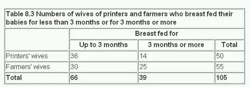
Clearly, we can see differences in counts/proportions of women who breast-fed their babies for three months or more, based on whether they were “printers wives” or “farmers’ wives”!

Is there a doctor in the House?

The CLT for Two Proportions

We first need to establish some model assumptions prior to making our analysis. As before, we wish to see if the CLT applies here, and if so, in what form. The difference between two proportions $\hat{p_{1}} - \hat{p_{2}}$ can be modeled using a normal distribution when:

Independence (extended): The data are independent within and between the two groups. Generally this is satisfied if the data come from two independent random samples or if the data come from a randomized experiment.
Success-failure condition: The success-failure condition holds for both groups, where we check successes and failures in each group separately. That is, we should have at least 10 successes and 10 failures in each of the two groups.

When these conditions are satisfied, the standard error of $\hat{p_{1}} - \hat{p_{2}}$ is well-approximated by:

$S E (\hat{p_{1}} - \hat{p_{2}}) = \sqrt{\frac{\hat{p_{1}} * (1 - \hat{p_{1}})}{n_{1}}} + \sqrt{\frac{\hat{p_{2}} * (1 - \hat{p_{2}})}{n_{2}}}$

where $\hat{p_{1}}$ and $\hat{p_{2}}$ represent the sample proportions, and $n_{1}$ and $n_{2}$ represent the sample sizes.

We can represent the Confidence Intervals as:

$\begin{array}{rcl} C I (p_{1} - p_{2}) & = & (\hat{p_{1}} - \hat{p_{2}}) \pm 1.96 * S E (\hat{p_{1}} - \hat{p_{2}}) \\ = & (\hat{p_{1}} - \hat{p_{2}}) \pm 1.96 * (\sqrt{\frac{\hat{p_{1}} * (1 - \hat{p_{1}})}{n_{1}}} + \sqrt{\frac{\hat{p_{2}} * (1 - \hat{p_{2}})}{n_{2}}}) \end{array}$

Case Study-1: `GSS2002` dataset

We saw how we could perform inference for a single proportion. We can extend this idea to multiple proportions too.

Let us try a dataset with Qualitative / Categorical data. This is the General Social Survey GSS dataset from the resampledata package, and we have people with different levels of Education stating their opinion on the Death Penalty. We want to know if these two Categorical variables have a correlation, i.e. can the opinions in favour of the Death Penalty be explained by the Education level?

Since data is Categorical ( both variables ), we need to take counts in a table, and then implement a chi-square test. In the test, we will permute the Education variable to see if we can see how significant its effect size is.

data(GSS2002, package = "resampledata")
glimpse(GSS2002)

Rows: 2,765
Columns: 21
$ ID            <int> 1, 2, 3, 4, 5, 6, 7, 8, 9, 10, 11, 12, 13, 14, 15, 16, 1…
$ Region        <fct> South Central, South Central, South Central, South Centr…
$ Gender        <fct> Female, Male, Female, Female, Male, Male, Female, Female…
$ Race          <fct> White, White, White, White, White, White, White, White, …
$ Education     <fct> HS, Bachelors, HS, Left HS, Left HS, HS, Bachelors, HS, …
$ Marital       <fct> Divorced, Married, Separated, Divorced, Divorced, Divorc…
$ Religion      <fct> Inter-nondenominational, Protestant, Protestant, Protest…
$ Happy         <fct> Pretty happy, Pretty happy, NA, NA, NA, Pretty happy, NA…
$ Income        <fct> 30000-34999, 75000-89999, 35000-39999, 50000-59999, 4000…
$ PolParty      <fct> "Strong Rep", "Not Str Rep", "Strong Rep", "Ind, Near De…
$ Politics      <fct> Conservative, Conservative, NA, NA, NA, Conservative, NA…
$ Marijuana     <fct> NA, Not legal, NA, NA, NA, NA, NA, NA, Legal, NA, NA, NA…
$ DeathPenalty  <fct> Favor, Favor, NA, NA, NA, Favor, NA, NA, Favor, NA, NA, …
$ OwnGun        <fct> No, Yes, NA, NA, NA, Yes, NA, NA, Yes, NA, NA, NA, NA, N…
$ GunLaw        <fct> Favor, Oppose, NA, NA, NA, Oppose, NA, NA, Oppose, NA, N…
$ SpendMilitary <fct> Too little, About right, NA, About right, NA, Too little…
$ SpendEduc     <fct> Too little, Too little, NA, Too little, NA, Too little, …
$ SpendEnv      <fct> About right, About right, NA, Too little, NA, Too little…
$ SpendSci      <fct> About right, About right, NA, Too little, NA, Too little…
$ Pres00        <fct> Bush, Bush, Bush, NA, NA, Bush, Bush, Bush, Bush, NA, NA…
$ Postlife      <fct> Yes, Yes, NA, NA, NA, Yes, NA, NA, Yes, NA, NA, NA, NA, …

inspect(GSS2002)


categorical variables:  
            name  class levels    n missing
1         Region factor      7 2765       0
2         Gender factor      2 2765       0
3           Race factor      3 2765       0
4      Education factor      5 2760       5
5        Marital factor      5 2765       0
6       Religion factor     13 2746      19
7          Happy factor      3 1369    1396
8         Income factor     24 1875     890
9       PolParty factor      8 2729      36
10      Politics factor      7 1331    1434
11     Marijuana factor      2  851    1914
12  DeathPenalty factor      2 1308    1457
13        OwnGun factor      3  924    1841
14        GunLaw factor      2  916    1849
15 SpendMilitary factor      3 1324    1441
16     SpendEduc factor      3 1343    1422
17      SpendEnv factor      3 1322    1443
18      SpendSci factor      3 1266    1499
19        Pres00 factor      5 1749    1016
20      Postlife factor      2 1211    1554
                                    distribution
1  North Central (24.7%) ...                    
2  Female (55.6%), Male (44.4%)                 
3  White (79.1%), Black (14.8%) ...             
4  HS (53.8%), Bachelors (16.1%) ...            
5  Married (45.9%), Never Married (25.6%) ...   
6  Protestant (53.2%), Catholic (24.5%) ...     
7  Pretty happy (57.3%) ...                     
8  40000-49999 (9.1%) ...                       
9  Ind (19.3%), Not Str Dem (18.9%) ...         
10 Moderate (39.2%), Conservative (15.8%) ...   
11 Not legal (64%), Legal (36%)                 
12 Favor (68.7%), Oppose (31.3%)                
13 No (65.5%), Yes (33.5%) ...                  
14 Favor (80.5%), Oppose (19.5%)                
15 About right (46.5%) ...                      
16 Too little (73.9%) ...                       
17 Too little (60%) ...                         
18 About right (49.7%) ...                      
19 Bush (50.6%), Gore (44.7%) ...               
20 Yes (80.5%), No (19.5%)                      

quantitative variables:  
  name   class min  Q1 median   Q3  max mean       sd    n missing
1   ID integer   1 692   1383 2074 2765 1383 798.3311 2765       0

skimr::skim(GSS2002)

Data summary
Name	GSS2002
Number of rows	2765
Number of columns	21
_______________________
Column type frequency:
factor	20
numeric	1
________________________
Group variables	None

Variable type: factor

skim_variable	n_missing	complete_rate	ordered	n_unique	top_counts
Region	0	1.00	FALSE	7	Nor: 684, Sou: 486, Sou: 471, Mid: 435
Gender	0	1.00	FALSE	2	Fem: 1537, Mal: 1228
Race	0	1.00	FALSE	3	Whi: 2188, Bla: 410, Oth: 167
Education	5	1.00	FALSE	5	HS: 1485, Bac: 443, Lef: 400, Gra: 230
Marital	0	1.00	FALSE	5	Mar: 1269, Nev: 708, Div: 445, Wid: 247
Religion	19	0.99	FALSE	13	Pro: 1460, Cat: 673, Non: 379, Chr: 65
Happy	1396	0.50	FALSE	3	Pre: 784, Ver: 415, Not: 170
Income	890	0.68	FALSE	24	400: 170, 300: 166, 250: 140, 500: 136
PolParty	36	0.99	FALSE	8	Ind: 528, Not: 515, Not: 449, Str: 408
Politics	1434	0.48	FALSE	7	Mod: 522, Con: 210, Sli: 209, Sli: 159
Marijuana	1914	0.31	FALSE	2	Not: 545, Leg: 306
DeathPenalty	1457	0.47	FALSE	2	Fav: 899, Opp: 409
OwnGun	1841	0.33	FALSE	3	No: 605, Yes: 310, Ref: 9
GunLaw	1849	0.33	FALSE	2	Fav: 737, Opp: 179
SpendMilitary	1441	0.48	FALSE	3	Abo: 615, Too: 414, Too: 295
SpendEduc	1422	0.49	FALSE	3	Too: 992, Abo: 278, Too: 73
SpendEnv	1443	0.48	FALSE	3	Too: 793, Abo: 439, Too: 90
SpendSci	1499	0.46	FALSE	3	Abo: 629, Too: 461, Too: 176
Pres00	1016	0.63	FALSE	5	Bus: 885, Gor: 781, Nad: 57, Oth: 16
Postlife	1554	0.44	FALSE	2	Yes: 975, No: 236

Variable type: numeric

skim_variable	n_missing	complete_rate	mean	sd	p0	p25	p50	p75	p100	hist
ID	0	1	1383	798.33	1	692	1383	2074	2765	▇▇▇▇▇

Note how all variables are Categorical !! Education has five levels, and of course DeathPenalty has three:

GSS2002 %>% count(Education)

ABCDEFGHIJ0123456789

Education <fct>	n <int>
NA	5
Left HS	400
HS	1485
Jr Col	202
Bachelors	443
Graduate	230

GSS2002 %>% count(DeathPenalty)

ABCDEFGHIJ0123456789

DeathPenalty <fct>	n <int>
NA	1457
Favor	899
Oppose	409

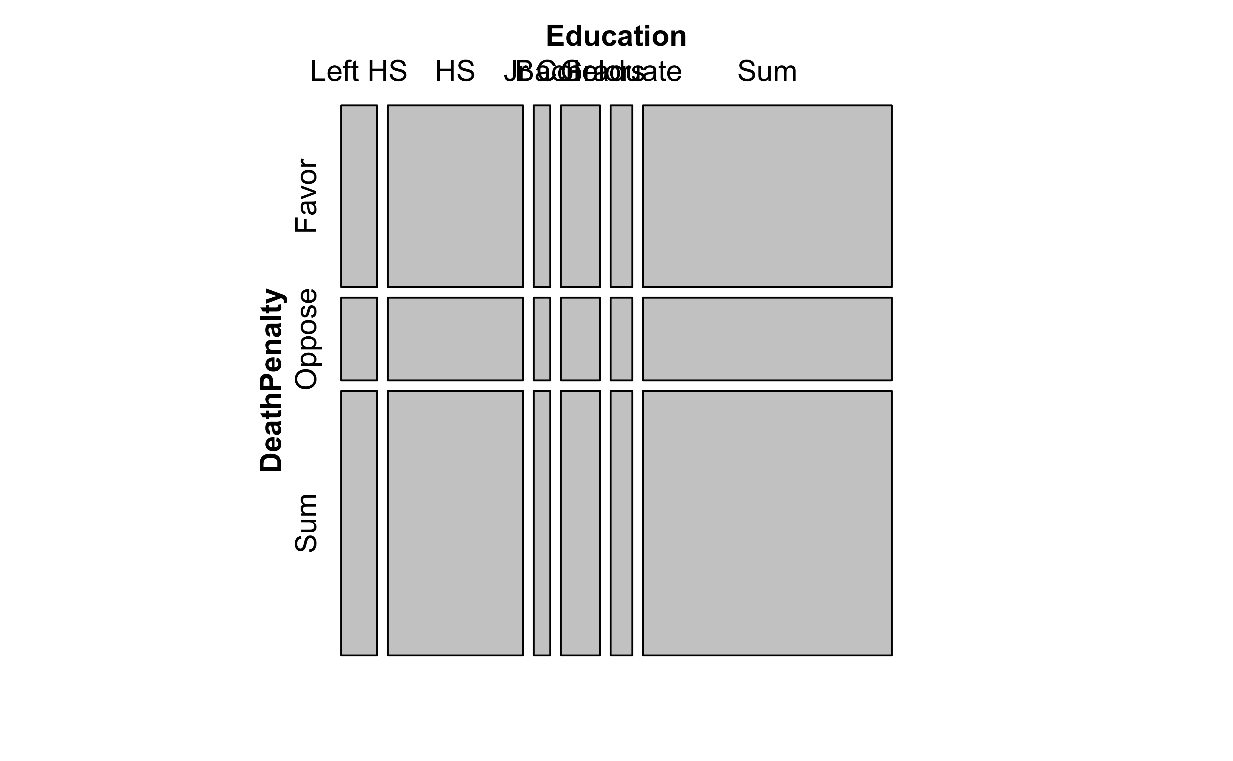
Let us drop NA entries in Education and Death Penalty and set up a Contingency Table.

gss2002 <- GSS2002 %>%
  dplyr::select(Education, DeathPenalty) %>%
  tidyr::drop_na(., c(Education, DeathPenalty))
##
gss_table <- mosaic::tally(DeathPenalty ~ Education, data = gss2002) %>%
  addmargins()
gss_table

            Education
DeathPenalty Left HS   HS Jr Col Bachelors Graduate  Sum
      Favor      117  511     71       135       64  898
      Oppose      72  200     16        71       50  409
      Sum        189  711     87       206      114 1307

Contingency Table Plots

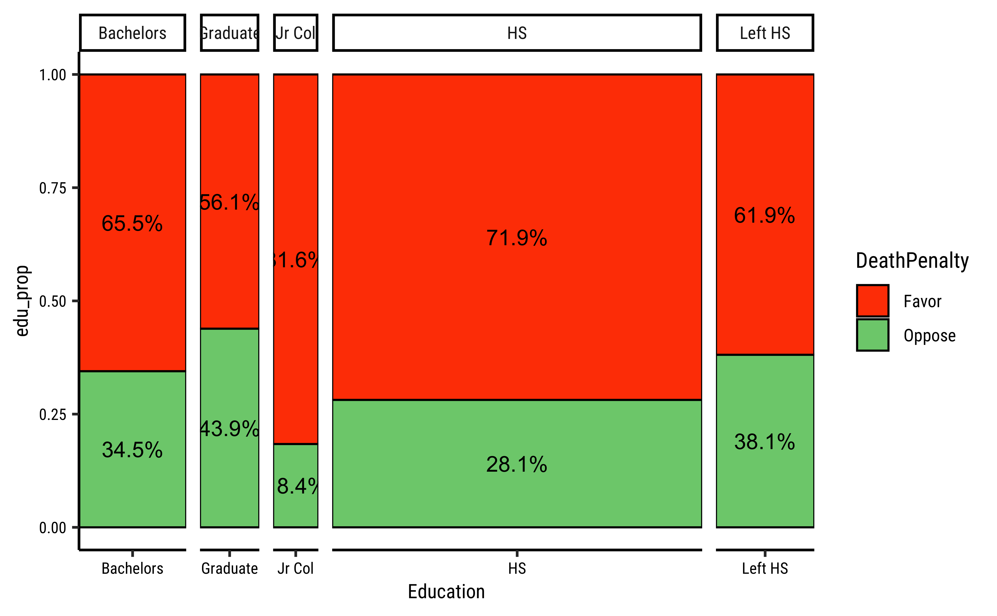
The Contingency Table can be plotted, as we have seen, using a mosaicplot using several packages. Let us do a quick recap:

mosaic::tally(DeathPenalty ~ Education, data = gss2002) %>%
  vcd::mosaic(gp = shading_hsv)

# library(ggmosaic)

# Set graph theme
theme_set(new = theme_custom())
#
ggplot(data = gss2002) +
  geom_mosaic(aes(
    x = product(DeathPenalty, Education),
    fill = DeathPenalty
  ))

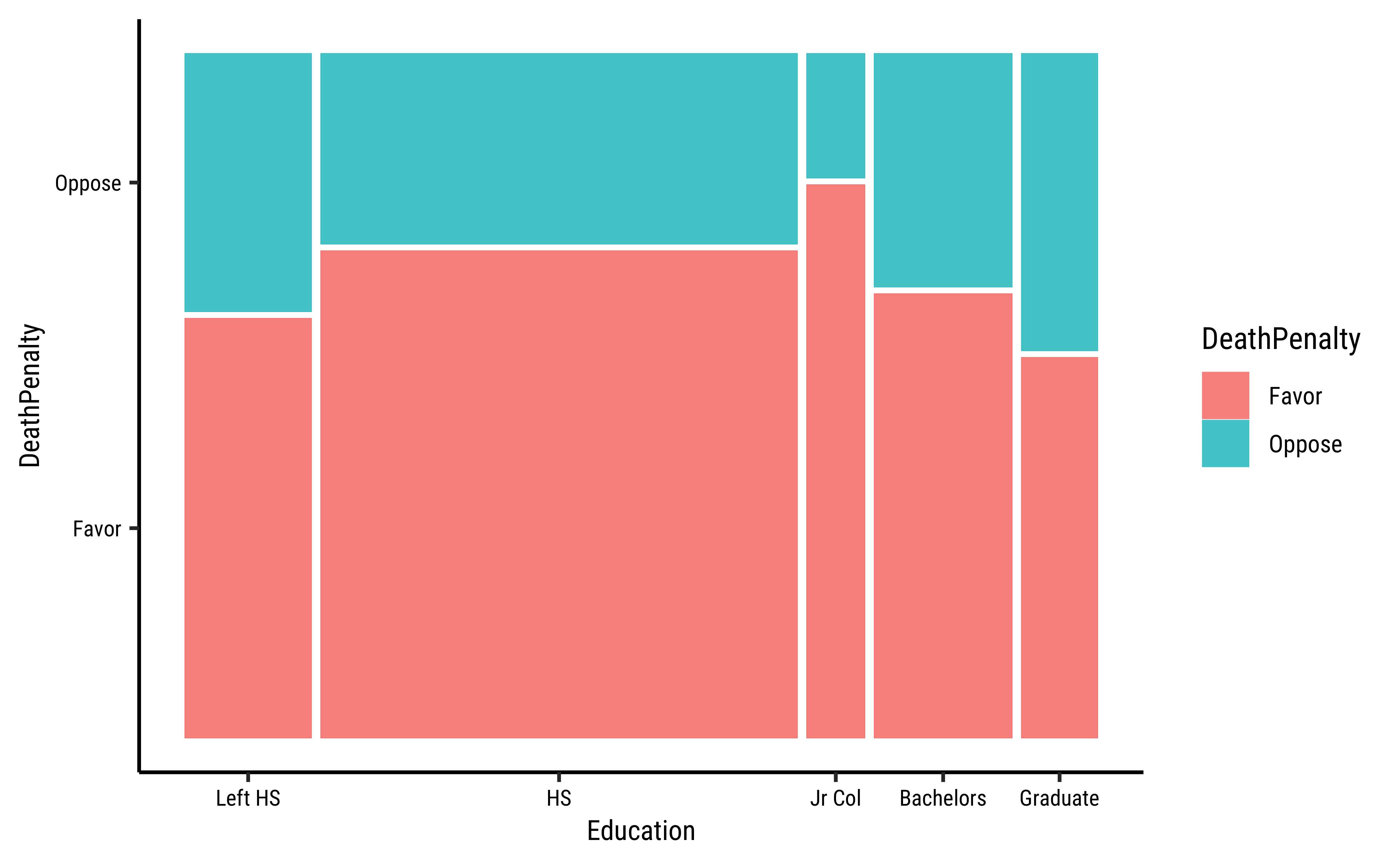
As seen before, it needs a little more work, to convert the Contingency Table into a tibble:

# https://stackoverflow.com/questions/19233365/how-to-create-a-marimekko-mosaic-plot-in-ggplot2

# Set graph theme
theme_set(new = theme_custom())
#

gss_summary <- gss2002 %>%
  mutate(
    Education = factor(
      Education,
      levels = c("Bachelors", "Graduate", "Jr Col", "HS", "Left HS"),
      labels = c("Bachelors", "Graduate", "Jr Col", "HS", "Left HS")
    ),
    DeathPenalty = as.factor(DeathPenalty)
  ) %>%
  group_by(Education, DeathPenalty) %>%
  summarise(count = n()) %>% # This is good for a chisq test

  # Add two more columns to facilitate mosaic/Marrimekko Plot
  mutate(
    edu_count = sum(count),
    edu_prop = count / sum(count)
  ) %>%
  ungroup()
###
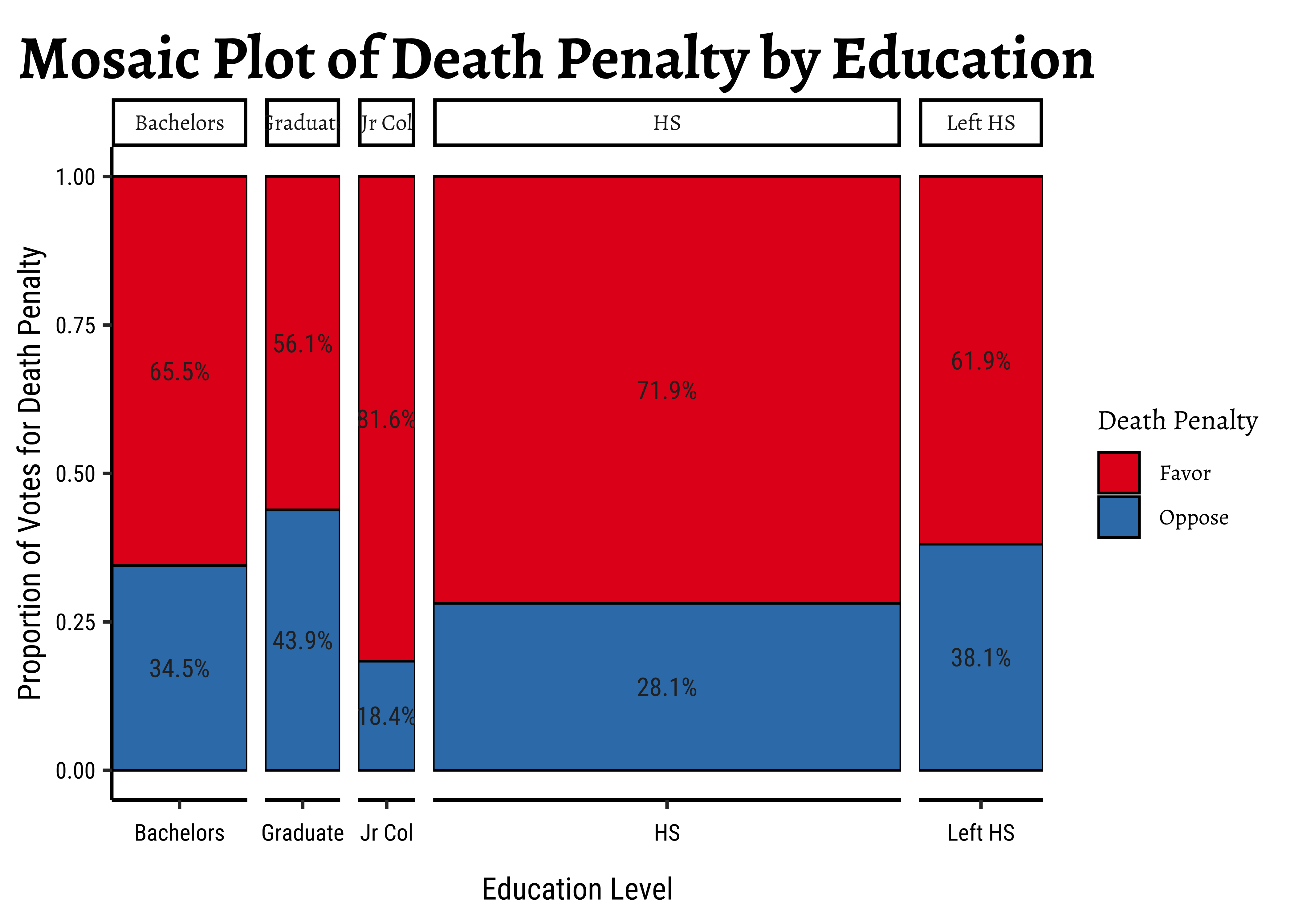
gf_col(edu_prop ~ Education,
  data = gss_summary,
  width = ~edu_count,
  fill = ~DeathPenalty,
  stat = "identity",
  position = "fill",
  color = "black"
) %>%
  gf_text(edu_prop ~ Education,
    label = ~ scales::percent(edu_prop),
    position = position_stack(vjust = 0.5)
  ) %>%
  gf_facet_grid(~Education,
    scales = "free_x",
    space = "free_x"
  ) %>%
  gf_theme(scale_fill_manual(values = c("orangered", "palegreen3")))

Hypotheses Definition

What would our Hypotheses be relating to the proportions of votes for or against the Death Penalty?

$H_{0} : Education does not affect votes for Death Penalty$

$H_{a} : Education affects votes for Death Penalty$

Inference for Two Proportions

We are now ready to perform our statistical inference. We will use the standard Pearson chi-square test, and develop and intuition for it. We will then do a permutation test to have an alternative method to complete the same task.

Code
Intuitive Explanation

Let us now perform the base chisq test: We need a contingency table and then the chisq test: We will calculate the observed-chi-squared value, and compare it with the critical value.

# Chi-square test
mosaic::xchisq.test(mosaic::tally(DeathPenalty ~ Education, data = gss2002))


    Pearson's Chi-squared test

data:  x
X-squared = 23.451, df = 4, p-value = 0.0001029

  117      511       71      135       64   
(129.86) (488.51) ( 59.78) (141.54) ( 78.33)
 [1.27]   [1.04]   [2.11]   [0.30]   [2.62] 
<-1.13>  < 1.02>  < 1.45>  <-0.55>  <-1.62> 
         
   72      200       16       71       50   
( 59.14) (222.49) ( 27.22) ( 64.46) ( 35.67)
 [2.79]   [2.27]   [4.63]   [0.66]   [5.75] 
< 1.67>  <-1.51>  <-2.15>  < 0.81>  < 2.40> 
         
key:
    observed
    (expected)
    [contribution to X-squared]
    <Pearson residual>

# Get the observed chi-square statistic
observedChi2 <- mosaic::chisq(mosaic::tally(DeathPenalty ~ Education, data = gss2002))
observedChi2

X.squared 
 23.45093

# Determine the Chi-Square critical value
X_squared_critical <- qchisq(
  p = .05,
  df = (5 - 1) * (2 - 1), # (nrows-1) * (ncols-1)
  lower.tail = FALSE
)
X_squared_critical

[1] 9.487729

We see that our observed $X^{2} = 23.45$ ; the critical value X_squared_critical is $9.48$ , which is much smaller! The p-value is $0.0001029$ , very low as we would expect, indicating that the NULL Hypothesis should be rejected in favour of the alternate hypothesis, that opinions about the DeathPenalty are related to Education.

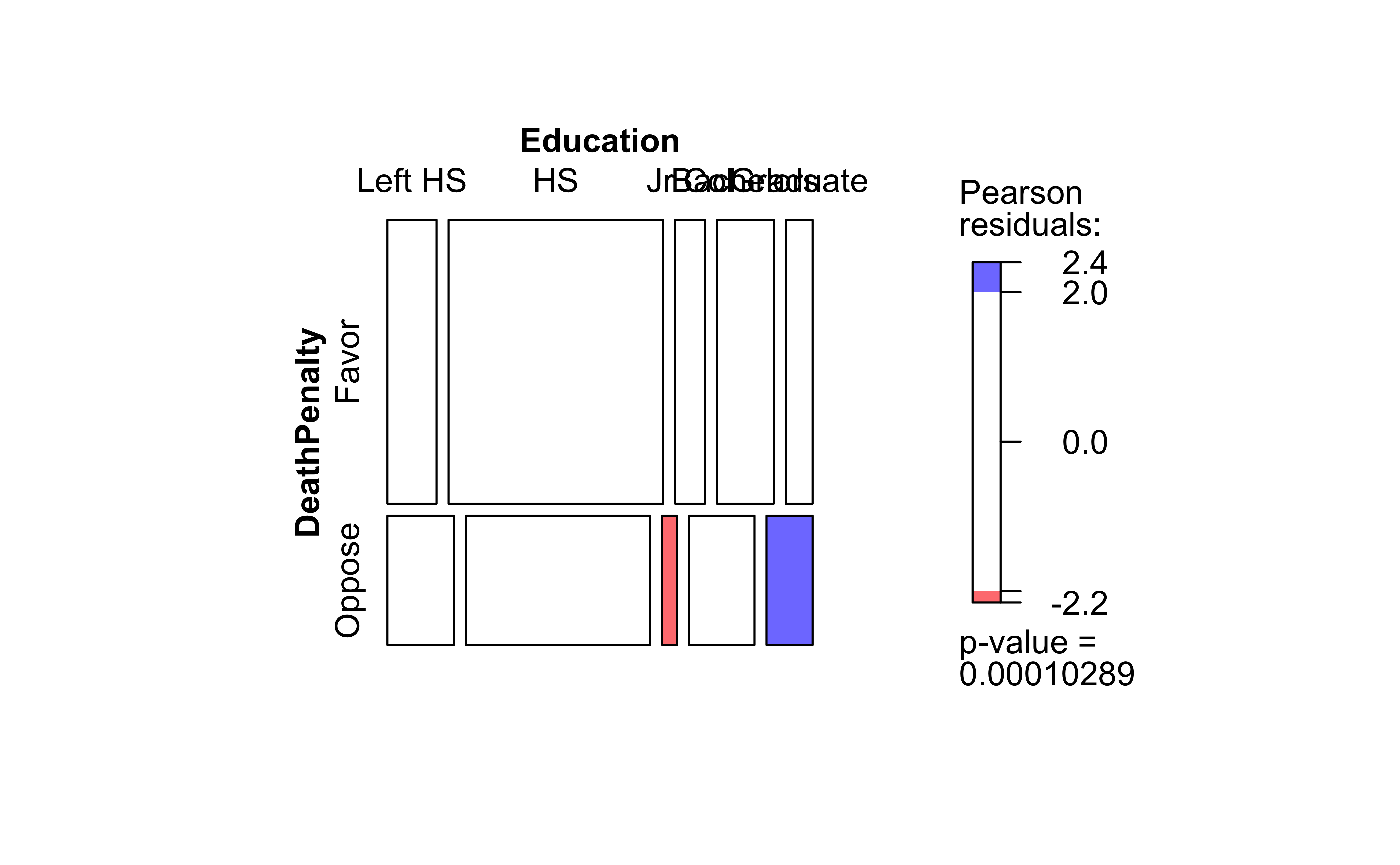
Verbose output not yet implemented.

Let us now dig into that cryptic-looking table above!

Let us look at the Contingency Table that we have:

DeathPenalty	Left HS	HS	Jr Col	Bachelors	Graduate	Sum
Favor	117	511	71	135	64	898
Oppose	72	200	16	71	50	409
Sum	189	711	87	206	114	1307

Figure 2: Contingency Table

In the chi-square test, we check whether the two (or more) categorical variables are independent. To do this we perform a simple check on the Contingency Table. We first re-compute the totals in each row and column, based on what we could expect if there was independence (NULL Hypothesis). If the two variables were independent, then there should be no difference between real and expected scores.

How do we know what scores to expect if there was no relationship between the variables?

Consider the entry in location (1,1): 117. The number of expected entries there is the probability of an entry landing in that square times the total number of entries:

$\begin{aligned} Expected Value[1,1] & = p_{r o w_{1}} * p_{c o l_{1}} * T o t a l S c o r e s \\ = \frac{\sum_{r_{1}}}{\sum_{r_{a l l} c_{a l l}}} * \frac{\sum_{c_{1}}}{\sum_{r_{a l l} c_{a l l}}} * \sum_{r_{a l l} c_{a l l}} \\ = \frac{898}{1307} * \frac{189}{1307} * 1307 \\ = 130 \end{aligned}$

Proceeding in this way for all the 15 entries in the Contingency Table, we get the “Expected” Contingency Table. Here are both tables for comparison:

Expected Contingency Table
	Left HS	HS	Jr Col	Bachelors	Graduate	Sum
Favor	130	489	60	142	78	898
Oppose	59	222	27	64	36	409
Sum	189	711	87	206	114	1307

Actual Contingency Table
	Left HS	HS	Jr Col	Bachelors	Graduate	Sum
Favor	117	511	71	135	64	898
Oppose	72	200	16	71	50	409
Sum	189	711	87	206	114	1307

And here are the mosaic plots for the actual and expected Contingency Tables, along with the association plot showing the differences, as we did when plotting Proportions:

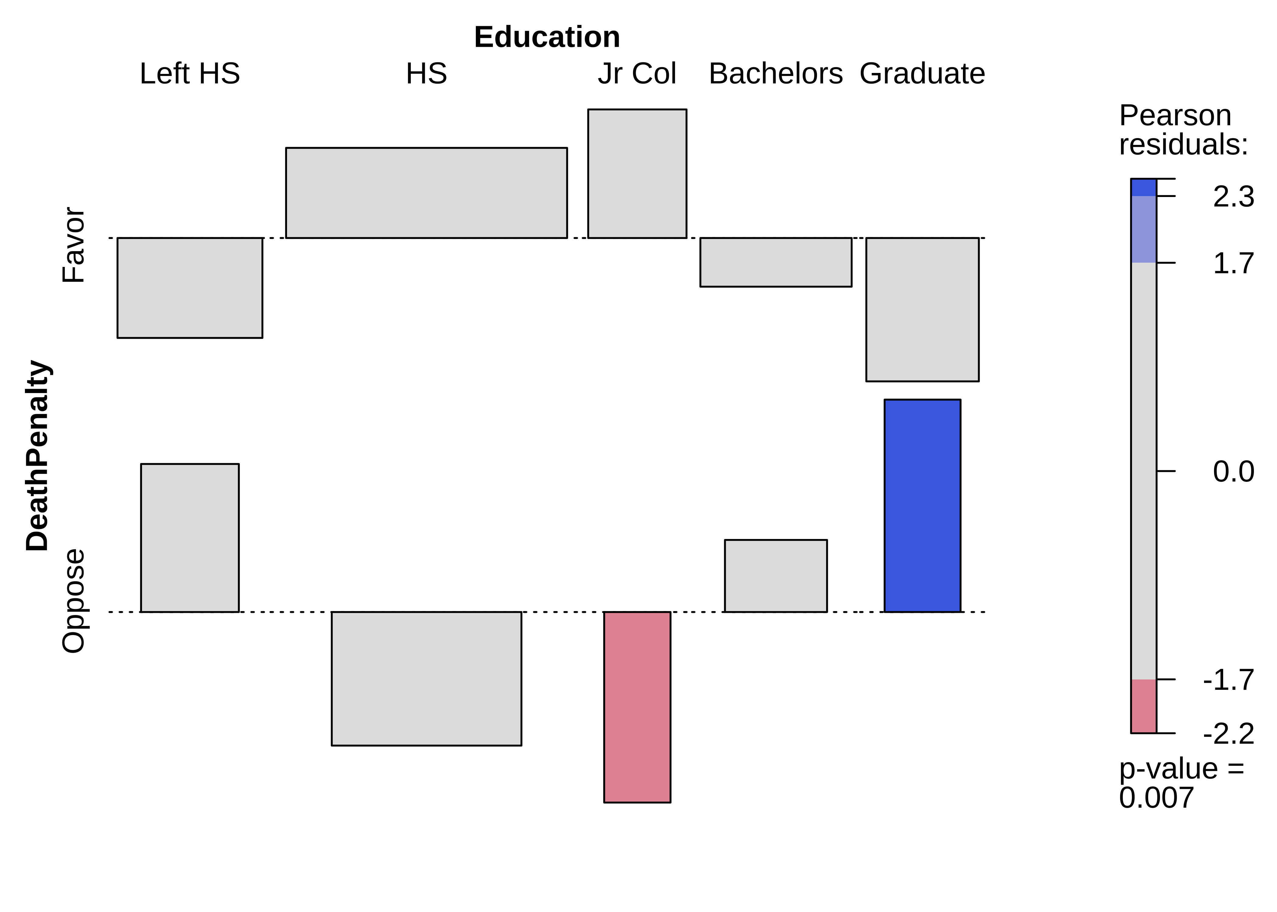
Now, the Pearson Residual in each cell is equivalent to the z-score of that cell. Recall the z-score idea: we subtract the mean and divide by the std. deviation to get the z-score.

In the Contingency Table, we have counts which are usually modeled as an (integer) Poisson distribution, for which mean (i.e Expected value) and variance are identical. Thus we get the Pearson Residual as:

$r_{i, j} = \frac{(A c t u a l - E x p e c t e d)}{\sqrt{E x p e c t e d}}$

and therefore:

$r_{i, j} = \frac{(o_{i, j} - e_{i, j})}{\sqrt{e_{i, j}}}$

The sum of all the squared Pearson residuals is the chi-square statistic, χ2, upon which the inferential analysis follows.

$χ 2 = \sum_{i = 1}^{R} \sum_{j = 1}^{C} r_{i, j}^{2}$

where R and C are number of rows and columns in the Contingency Table, the levels in the two Qual variables.

For location [1,1], its contribution to χ2 would be: $(117 - 130)^{2} / 130 = 1.3$ . Do try to compute all of these and the $X^{2}$ statistic by hand !!

All right, what of all this? How did this $X^{2}$ distribution come from? Here is a lovely, brief explanation from this StackOverflow Post:

In a Contingency Table the Null Hypothesis states that the variables in the rows and the variable in the columns are independent.

The cell counts $E_{i j}$ are assumed to be Poisson distributed with mean = $E_{i j}$ and as they are Poisson, their variance is also $E_{i j}$ .

Asymptotically the Poisson distribution approaches the normal distribution, with mean = $E_{i j}$ and standard deviation with $\sqrt{E_{i j}}$ so, asymptotically $\frac{(X_{i j} - E_{i j})}{\sqrt{E_{i j}}}$ is approximately standard normal $N (0, 1)$ .

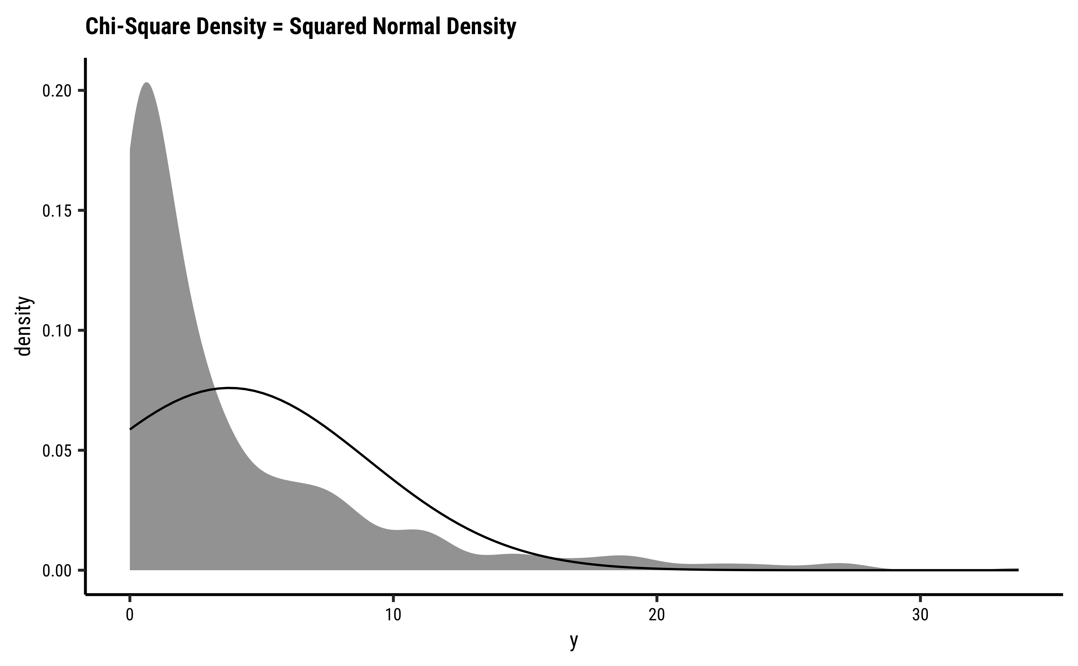
If you square standard normal variables and sum these squares then the result is a chi-square random variable so $\sum_{i, j} {(\frac{(X_{i j} - E_{i j})}{\sqrt{E_{i j}}})}^{2}$ has a (asymptotically) a chi-square distribution.

Asymptotics must hold and that is why most textbooks state that the result of the test is valid when all expected cell counts $E_{i j}$ are larger than 5, but that is just a rule of thumb that makes the approximation ‘’good enough’’.

Permutation Test for `Education`

We will now perform the permutation test for the difference between proportions. We will first get an intuitive idea of the permutation, and then perform it using both mosaic and infer.

Permutation Visually Demonstrated
Code

We saw from the diagram created by Allen Downey that there is only one test! We will now use this philosophy to develop a technique that allows us to mechanize several Statistical Models in that way, with nearly identical code. We will first look visually at a permutation exercise. We will create dummy data that contains the following case study:

A set of identical resumes was sent to male and female evaluators. The candidates in the resumes were of both genders. We wish to see if there was difference in the way resumes were evaluated, by male and female evaluators. (We use just one male and one female evaluator here, to keep things simple!)

ABCDEFGHIJ0123456789

evaluator <fct>	candidate_selected <dbl>
F	1
F	1
F	1
F	1
F	1
F	1
F	1
F	1
F	0
F	1

ABCDEFGHIJ0123456789

evaluator <fct>	selection_ratio <dbl>	count <int>	n <int>
F	0.1250000	3	24
M	0.4583333	11	24

         M 
-0.3333333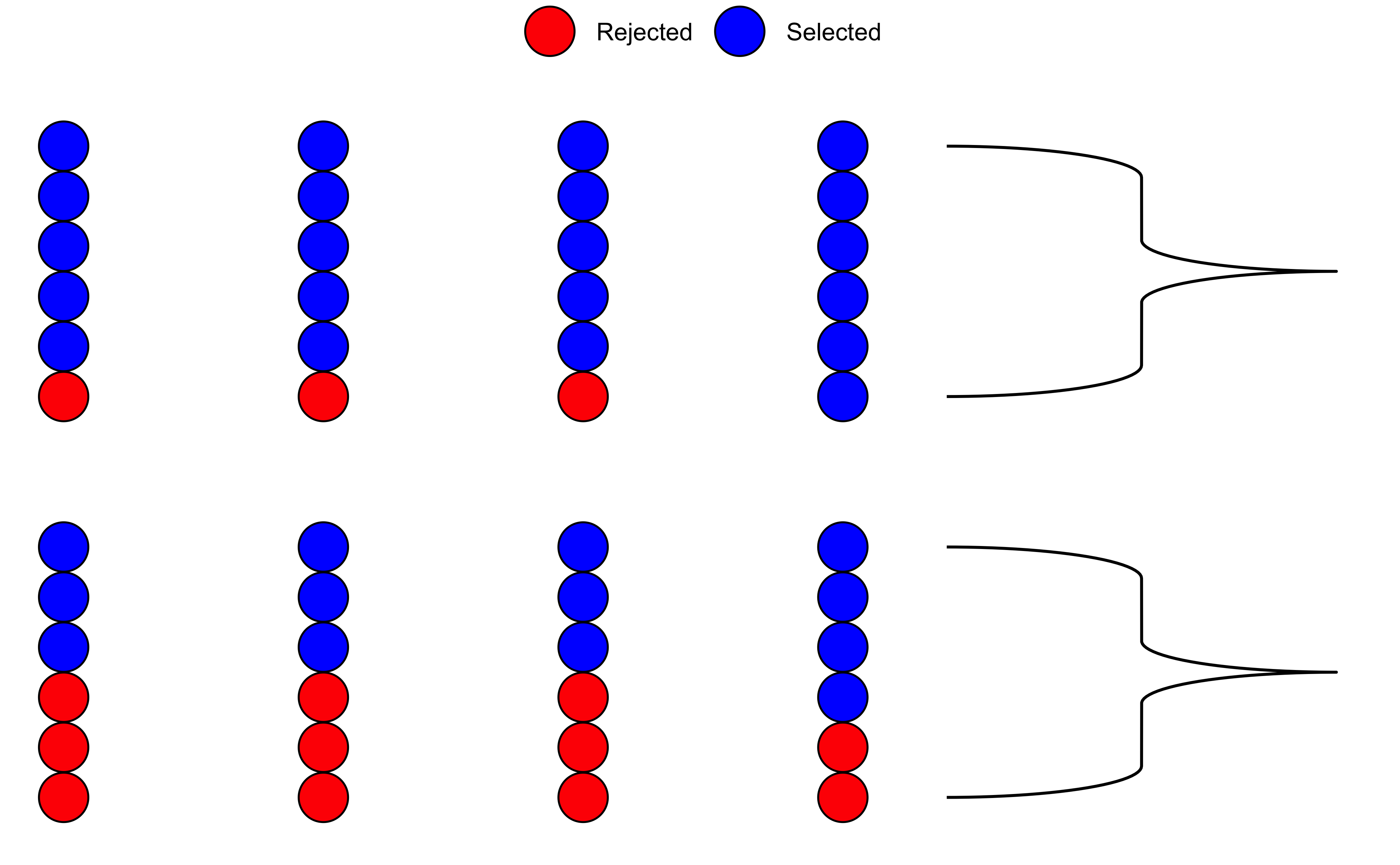

So, we have a solid disparity in percentage of selection between the two evaluators! Now we pretend that there is no difference between the selections made by either set of evaluators. So we can just:

Pool up all the evaluations
Arbitrarily re-assign a given candidate(selected or rejected) to either of the two sets of evaluators, by permutation.

How would that pooled shuffled set of evaluations look like?

ABCDEFGHIJ0123456789

selection_ratio <dbl>	count <int>	n <int>
0.2916667	14	48

As can be seen, the ratio is different!

We can now check out our Hypothesis that there is no bias. We can shuffle the data many many times, calculating the ratio each time, and plot the distribution of the differences in selection ratio and see how that artificially created distribution compares with the originally observed figure from Mother Nature.

# Set graph theme
theme_set(new = theme_custom())
#
null_dist <- do(4999) * diff(mean(
  candidate_selected ~ shuffle(evaluator),
  data = data
))
# null_dist %>% names()
null_dist %>%
  gf_histogram(~M,
    fill = ~ (M <= obs_difference),
    bins = 25, show.legend = FALSE,
    xlab = "Bias Proportion",
    ylab = "How Often?",
    title = "Permutation Test on Difference between Groups",
    subtitle = ""
  ) %>%
  gf_vline(xintercept = ~obs_difference, color = "red") %>%
  gf_label(500 ~ obs_difference,
    label = "Observed\n Bias",
    show.legend = FALSE
  )
mean(~ M <= obs_difference, data = null_dist)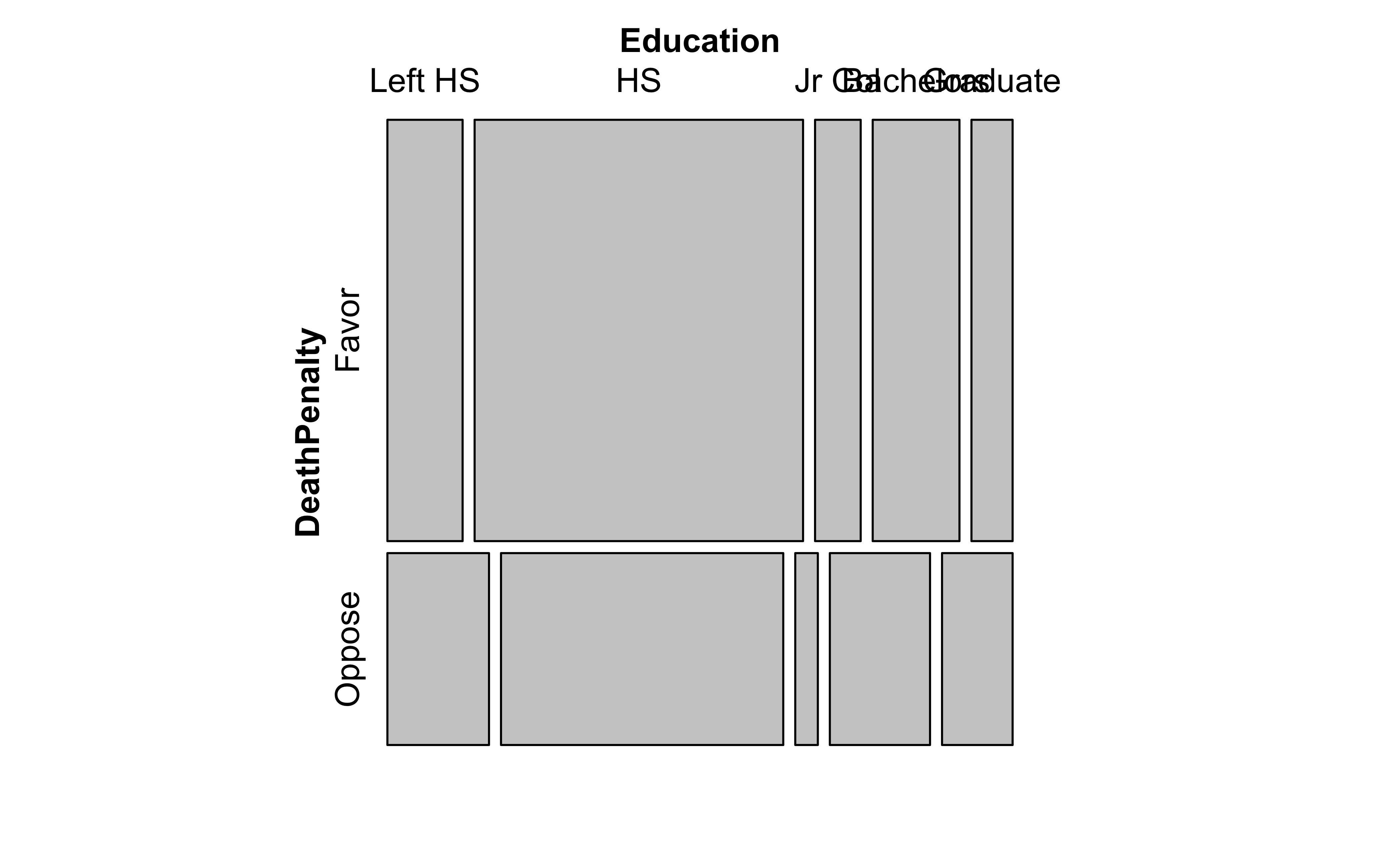

[1] 0.00220044

We see that the artificial data can hardly ever ( $p = 0.0022$ ) mimic what the real world experiment is showing. Hence we had good reason to reject our NULL Hypothesis that there is no bias.

We should now repeat the test with permutations on Education:

# Set graph theme
theme_set(new = theme_custom())
#

null_chisq <- do(4999) *
  chisq.test(mosaic::tally(DeathPenalty ~ shuffle(Education),
    data = gss2002
  ))

head(null_chisq)

ABCDEFGHIJ0123456789

	X.squared <dbl>	df <int>	p.value <dbl>	method <chr>
X-squared...1	12.319854	4	0.01512469	Pearson's Chi-squared test
X-squared...2	5.208442	4	0.26657081	Pearson's Chi-squared test
X-squared...3	5.431285	4	0.24583591	Pearson's Chi-squared test
X-squared...4	8.918993	4	0.06315646	Pearson's Chi-squared test
X-squared...5	1.251510	4	0.86954725	Pearson's Chi-squared test
X-squared...6	1.802120	4	0.77209444	Pearson's Chi-squared test

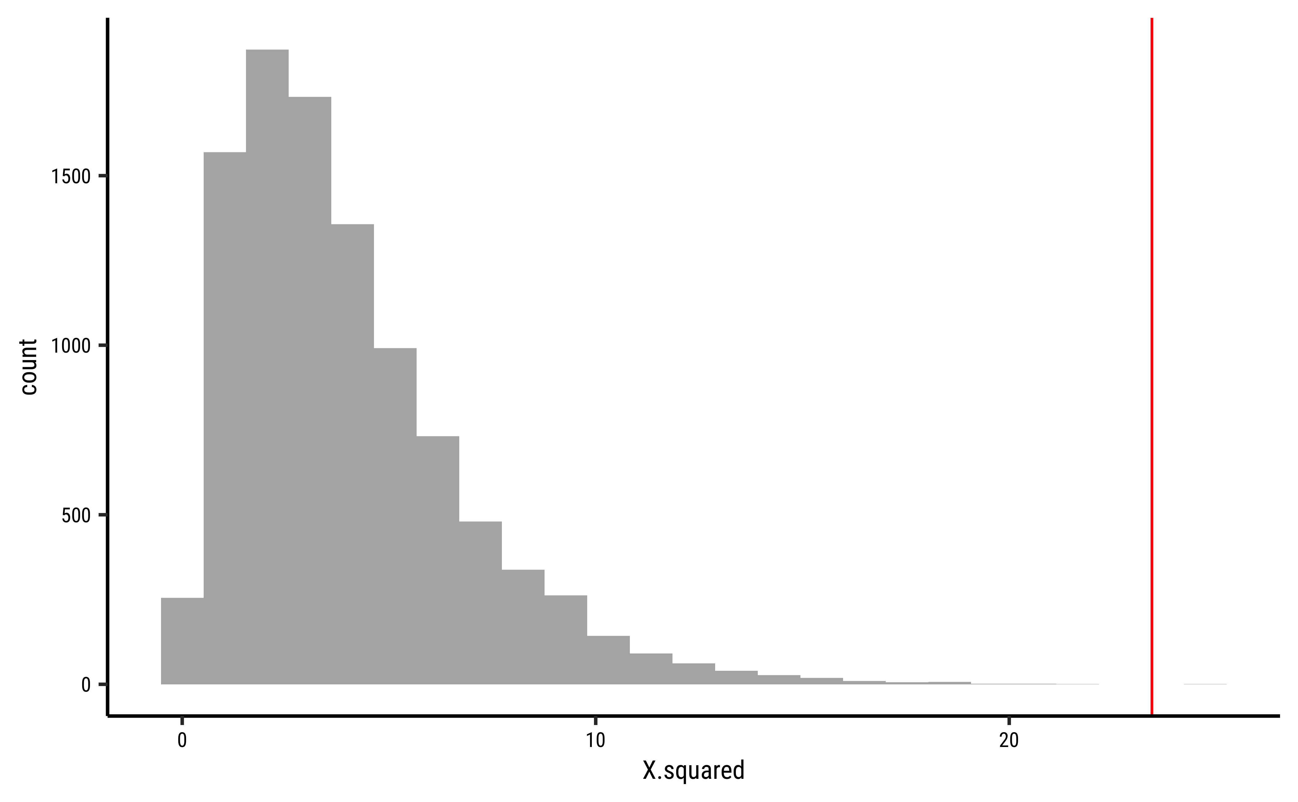
gf_histogram(~X.squared, data = null_chisq) %>%
  gf_vline(
    xintercept = observedChi2,
    color = "red"
  )

prop1(~ X.squared >= observedChi2, data = null_chisq)

prop_TRUE 
    2e-04

The p-value is well below our threshold of $0.05$ , so we would conclude that Education has a significant effect on DeathPenalty opinion!

Inference for Proportions Case Study-2: TBD dataset

To be Written Up.

Conclusion

In our basic $X^{2}$ test, we calculate the test statistic of $X^{2}$ and look up a theoretical null distribution for that statistic, and see how unlikely our observed value is.

Why would a permutation test be a good idea here? With a permutation test, there are no assumptions of the null distribution: this is computed based on real data. We note in passing that, in this case, since the number of cases in each cell of the Contingency Table are fairly high ( >= 5) the resulting NULL distribution is of the $X^{2}$ variety.

Wait, But Why?

Your Turn

References

OpenIntro Modern Statistics: Chapter 17
Chapter 8: The Chi-Square Test, from Statistics at Square One. The British Medical Journal. https://www.bmj.com/about-bmj/resources-readers/publications/statistics-square-one/8-chi-squared-tests. Very readable and easy to grasp. Especially if you like watching Grey’s Anatomy and House.
Exploring the underlying theory of the chi-square test through simulation - part 1 https://www.rdatagen.net/post/a-little-intuition-and-simulation-behind-the-chi-square-test-of-independence/
Exploring the underlying theory of the chi-square test through simulation - part 2 https://www.rdatagen.net/post/a-little-intuition-and-simulation-behind-the-chi-square-test-of-independence-part-2/
An Online $Ξ^{2}$ -test calculator. https://www.statology.org/chi-square-test-of-independence-calculator/
https://saylordotorg.github.io/text_introductory-statistics/s13-04-comparison-of-two-population-p.html

R Package Citations

Package	Version	Citation
ggmosaic	0.3.3	Jeppson, Hofmann, and Cook (2021)
resampledata	0.3.2	Chihara and Hesterberg (2018)
scales	1.4.0	Wickham, Pedersen, and Seidel (2025)
vcd	1.4.13	Meyer, Zeileis, and Hornik (2006); Zeileis, Meyer, and Hornik (2007); Meyer et al. (2024)

Chihara, Laura M., and Tim C. Hesterberg. 2018. Mathematical Statistics with Resampling and r. John Wiley & Sons Hoboken NJ. https://github.com/lchihara/MathStatsResamplingR?tab=readme-ov-file.

Jeppson, Haley, Heike Hofmann, and Di Cook. 2021. ggmosaic: Mosaic Plots in the “ggplot2” Framework. https://doi.org/10.32614/CRAN.package.ggmosaic.

Meyer, David, Achim Zeileis, and Kurt Hornik. 2006. “The Strucplot Framework: Visualizing Multi-Way Contingency Tables with Vcd.” Journal of Statistical Software 17 (3): 1–48. https://doi.org/10.18637/jss.v017.i03.

Meyer, David, Achim Zeileis, Kurt Hornik, and Michael Friendly. 2024. vcd: Visualizing Categorical Data. https://doi.org/10.32614/CRAN.package.vcd.

Wickham, Hadley, Thomas Lin Pedersen, and Dana Seidel. 2025. scales: Scale Functions for Visualization. https://doi.org/10.32614/CRAN.package.scales.

Zeileis, Achim, David Meyer, and Kurt Hornik. 2007. “Residual-Based Shadings for Visualizing (Conditional) Independence.” Journal of Computational and Graphical Statistics 16 (3): 507–25. https://doi.org/10.1198/106186007X237856.

Citation

BibTeX citation:

@online{v.2022,
  author = {V., Arvind},
  title = {🃏 {Inference} {Test} for {Two} {Proportions}},
  date = {2022-11-10},
  url = {https://av-quarto.netlify.app/content/courses/Analytics/Inference/Modules/190-TwoProp/},
  langid = {en},
  abstract = {Inference Test for Two Proportions}
}

For attribution, please cite this work as:

V., Arvind. 2022. “🃏 Inference Test for Two Proportions.” November 10, 2022. https://av-quarto.netlify.app/content/courses/Analytics/Inference/Modules/190-TwoProp/.

Setting up R packages

Plot Theme

Introduction

The CLT for Two Proportions

Case Study-1: GSS2002 dataset

Contingency Table Plots

Hypotheses Definition

Inference for Two Proportions

Permutation Test for Education

Inference for Proportions Case Study-2: TBD dataset

Conclusion

Wait, But Why?

Your Turn

References

R Package Citations

Citation

Case Study-1: `GSS2002` dataset

Permutation Test for `Education`