Modelling with Logistic Regression
Plot Fonts and Theme
Show the Code
library(systemfonts)
library(showtext)
## Clean the slate
systemfonts::clear_local_fonts()
systemfonts::clear_registry()
##
showtext_opts(dpi = 96) # set DPI for showtext
sysfonts::font_add(
  family = "Alegreya",
  regular = "../../../../../../fonts/Alegreya-Regular.ttf",
  bold = "../../../../../../fonts/Alegreya-Bold.ttf",
  italic = "../../../../../../fonts/Alegreya-Italic.ttf",
  bolditalic = "../../../../../../fonts/Alegreya-BoldItalic.ttf"
)
Error in check_font_path(bold, "bold"): font file not found for 'bold' typeShow the Code
sysfonts::font_add(
  family = "Roboto Condensed",
  regular = "../../../../../../fonts/RobotoCondensed-Regular.ttf",
  bold = "../../../../../../fonts/RobotoCondensed-Bold.ttf",
  italic = "../../../../../../fonts/RobotoCondensed-Italic.ttf",
  bolditalic = "../../../../../../fonts/RobotoCondensed-BoldItalic.ttf"
)
showtext_auto(enable = TRUE) # enable showtext
##
theme_custom <- function() {
  font <- "Alegreya" # assign font family up front

  theme_classic(base_size = 14, base_family = font) %+replace% # replace elements we want to change

    theme(
      text = element_text(family = font), # set base font family

      # text elements
      plot.title = element_text( # title
        family = font, # set font family
        size = 24, # set font size
        face = "bold", # bold typeface
        hjust = 0, # left align
        margin = margin(t = 5, r = 0, b = 5, l = 0)
      ), # margin
      plot.title.position = "plot",
      plot.subtitle = element_text( # subtitle
        family = font, # font family
        size = 14, # font size
        hjust = 0, # left align
        margin = margin(t = 5, r = 0, b = 10, l = 0)
      ), # margin

      plot.caption = element_text( # caption
        family = font, # font family
        size = 9, # font size
        hjust = 1
      ), # right align

      plot.caption.position = "plot", # right align

      axis.title = element_text( # axis titles
        family = "Roboto Condensed", # font family
        size = 12
      ), # font size

      axis.text = element_text( # axis text
        family = "Roboto Condensed", # font family
        size = 9
      ), # font size

      axis.text.x = element_text( # margin for axis text
        margin = margin(5, b = 10)
      )

      # since the legend often requires manual tweaking
      # based on plot content, don't define it here
    )
}
Show the Code
```{r}
#| cache: false
#| code-fold: true
## Set the theme
theme_set(new = theme_custom())

## Use available fonts in ggplot text geoms too!
update_geom_defaults(geom = "text", new = list(
  family = "Roboto Condensed",
  face = "plain",
  size = 3.5,
  color = "#2b2b2b"
))
```
Sometimes the dependent variable is Qualitative: an either/or categorization. for example, or the variable we want to predict might be won or lost the contest, has an ailment or not, voted or not in the last election, or graduated from college or not. There might even be more than two categories such as voted for Congress, BJP, or Independent; or never smoker, former smoker, or current smoker.
We saw with the General Linear Model that it models the mean of a target Quantitative variable as a linear weighted sum of the predictor variables:
This model is considered to be general because of the dependence on potentially more than one explanatory variable, v.s. the simple linear model:1
Although a very useful framework, there are some situations where general linear models are not appropriate:
- the range of Y is restricted (e.g. binary, count)
- the variance of Y depends on the mean (Taylor’s Law)2
How do we use the familiar linear model framework when the target/dependent variable is Categorical?
Linear Models for Categorical Targets?
Recall that we spoke of dummy-encoded Qualitative **predictor** variables for our linear models and how we would dummy encode them using numerical values, such as 0 and 1, or +1 and -1. Could we try the same way for a target categorical variable?
Sadly this seems to not work for categorical dependent variables using a simple linear model as before. Consider the Credit Card Default data from the package ISLR.
default <fct> | student <fct> | balance <dbl> | income <dbl> | default_yes <dbl> |
|---|---|---|---|---|
| No | No | 729.5264952 | 44361.6251 | 0 |
| No | Yes | 817.1804066 | 12106.1347 | 0 |
| No | No | 1073.5491640 | 31767.1389 | 0 |
| No | No | 529.2506047 | 35704.4939 | 0 |
| No | No | 785.6558829 | 38463.4959 | 0 |
| No | Yes | 919.5885305 | 7491.5586 | 0 |
| No | No | 825.5133305 | 24905.2266 | 0 |
| No | Yes | 808.6675043 | 17600.4513 | 0 |
| No | No | 1161.0578540 | 37468.5293 | 0 |
| No | No | 0.0000000 | 29275.2683 | 0 |
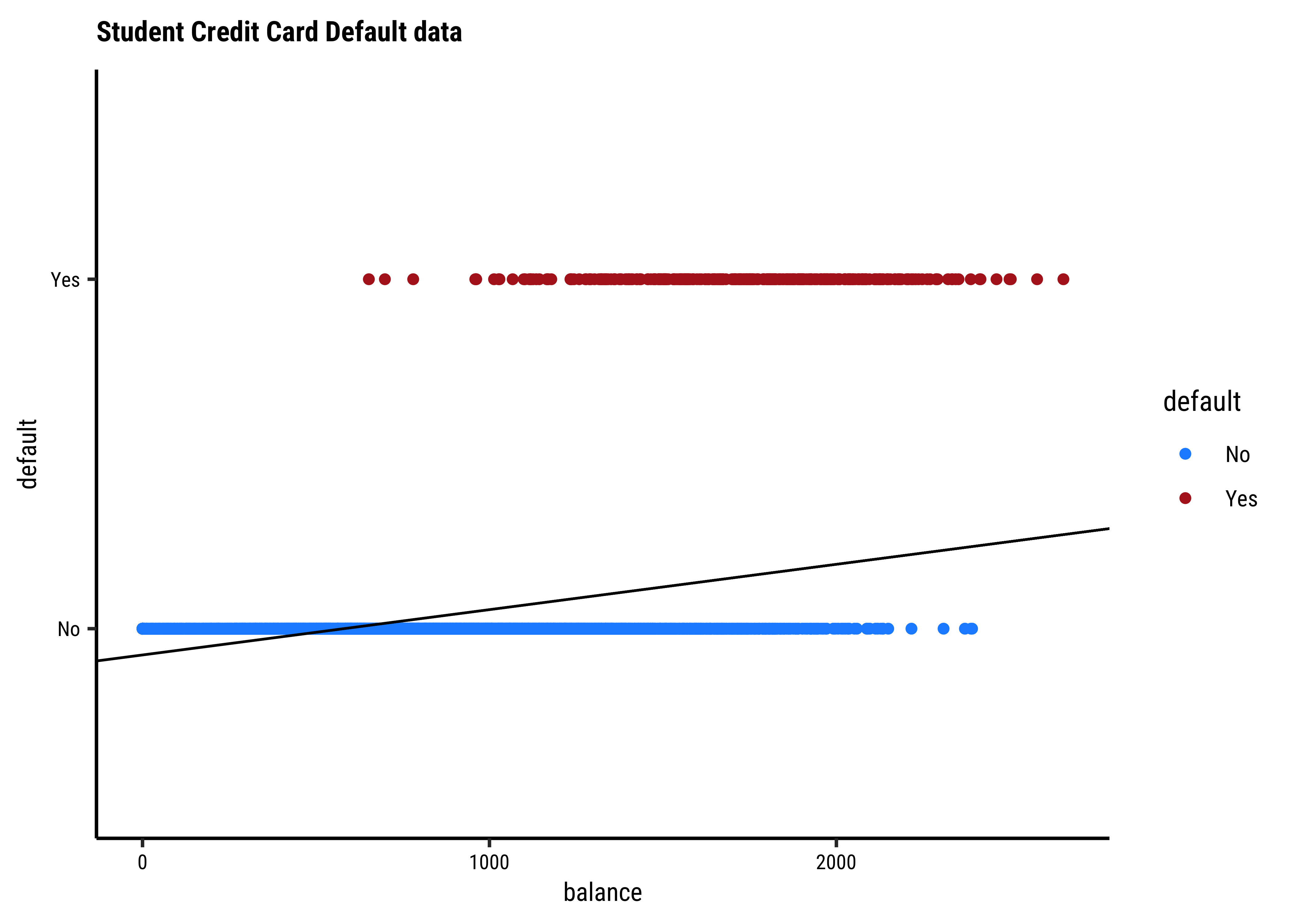
We see balance and income are quantitative predictors; student is a qualitative predictor, and default is a qualitative target variable. If we naively use a linear model equation as model = lm(default ~ balance, data = Default) and plot it, then…
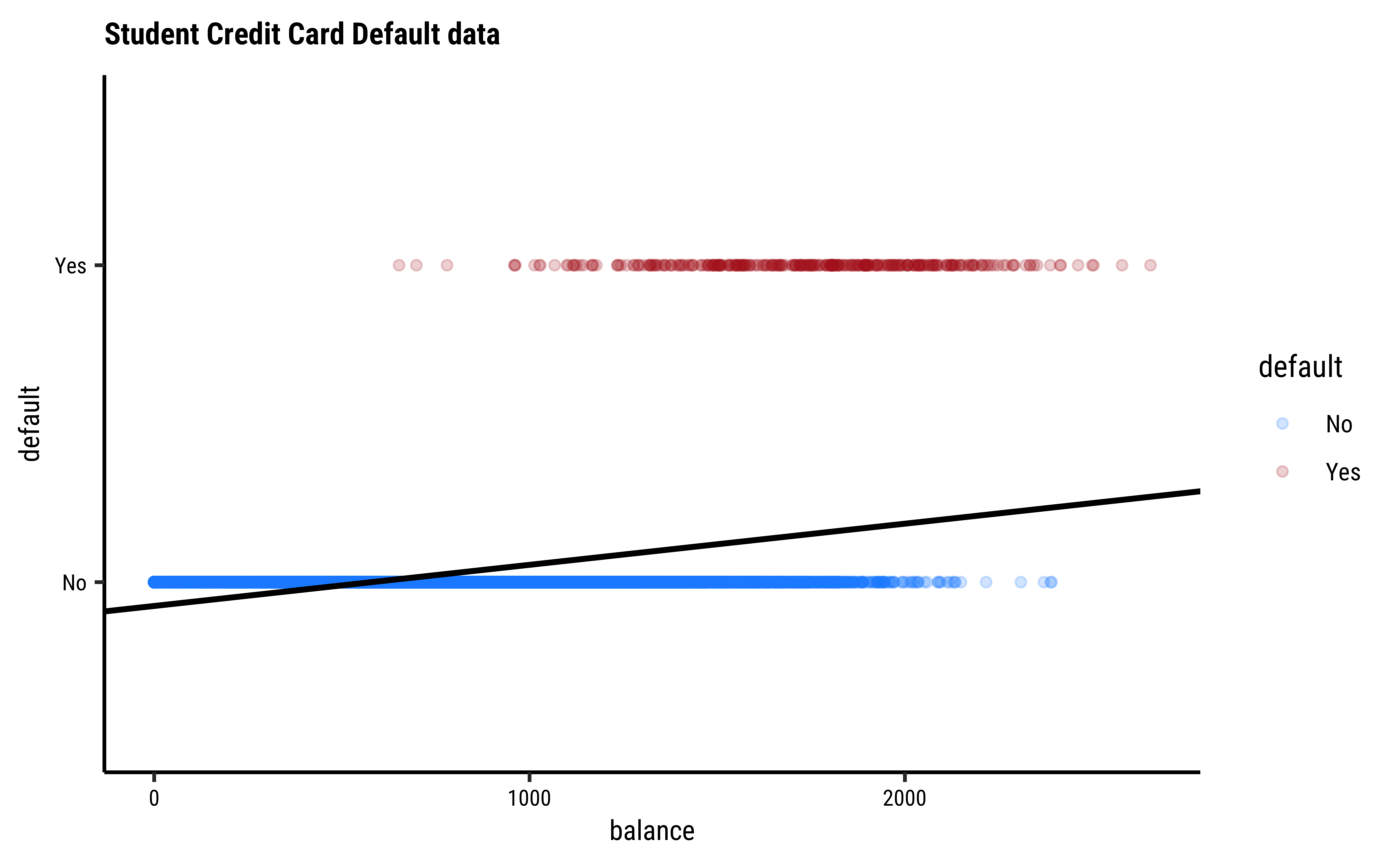
…it is pretty much clear from Figure 1 that something is very odd. (no pun intended! See below!) If the only possible values for default are
Where do we go from here?
Let us state what we might desire of our model:
-
Model Equation: Despite this setback, we would still like our model to be as close as possible to the familiar linear model equation.
Predictors and Weights: We have quantitative predictors so we still want to use a linear-weighted sum for the RHS (i.e predictor side) of the model equation. What can we try to make this work? Especially for the LHS (i.e the target side)?
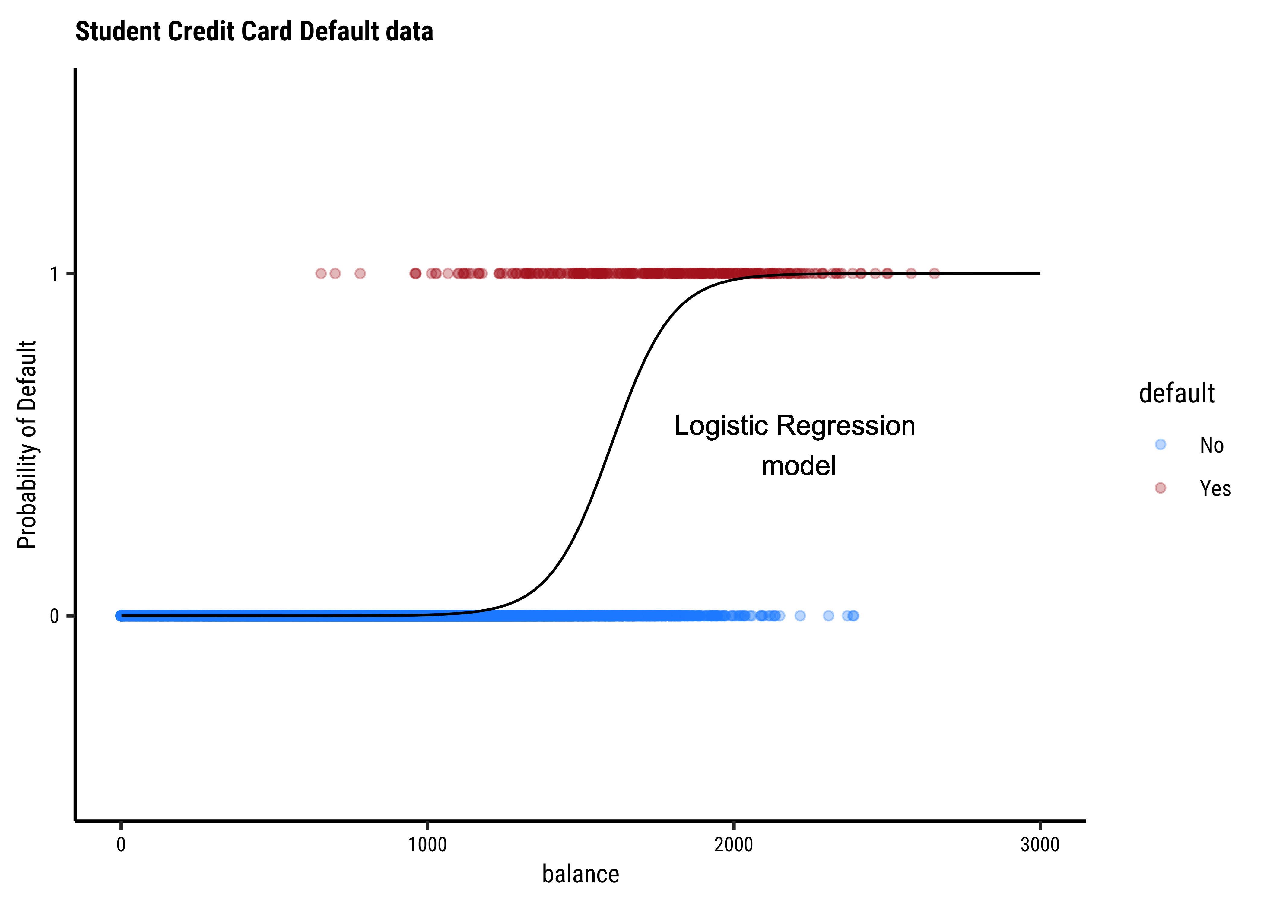
Making the LHS continuous: What can we try? In dummy encoding our target variable, we found a range of [0,1], which is the same range for a probability value! Could we try to use probability of the outcome as our target, even though we are interested in binary outcomes? This would still leave us with a range of
If we map our Categorical/Qualitative target variable into a Quantitative probability, we need immediately to look at the LINE assumptions in linear regression.
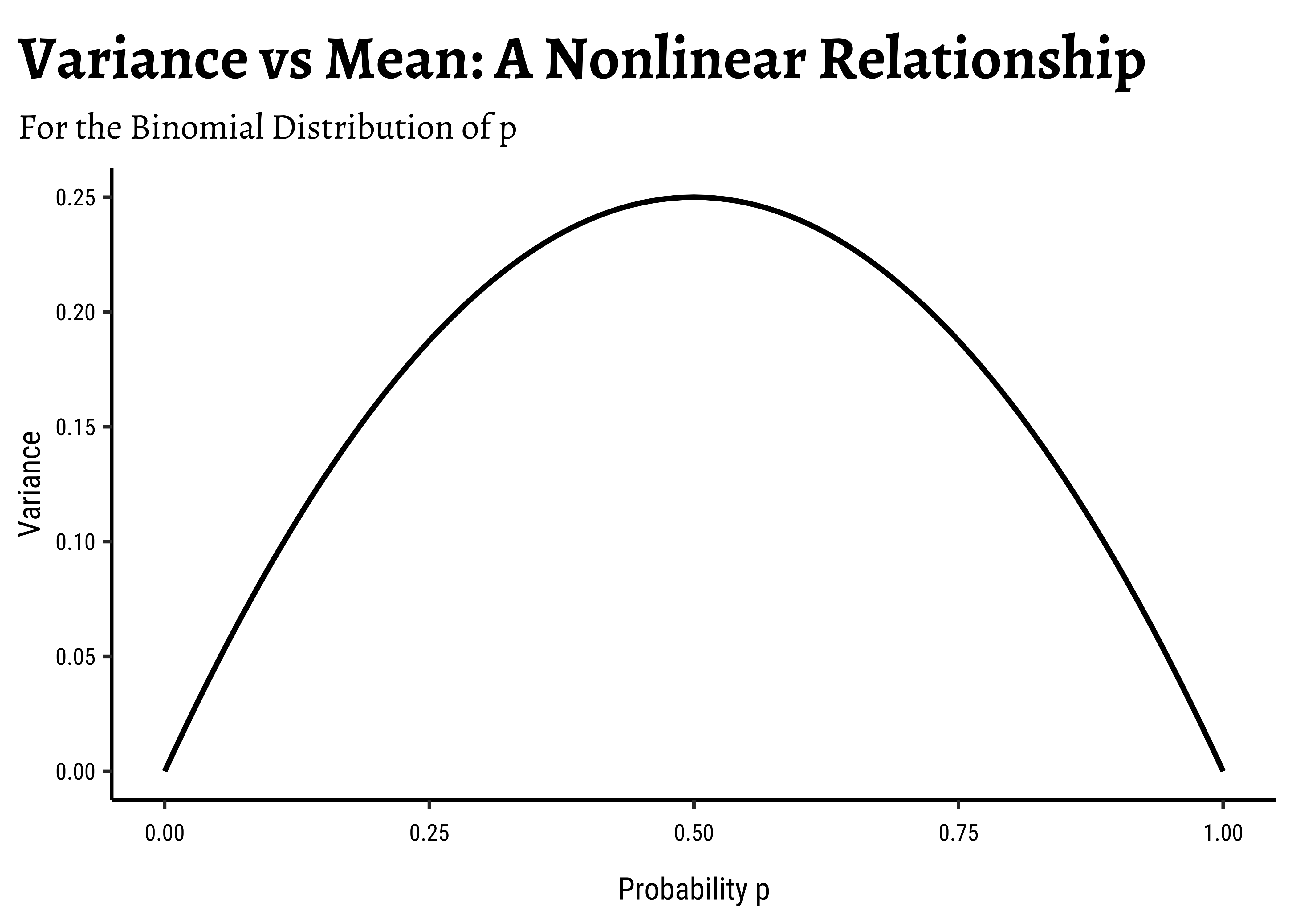
In linear regression, we assume a normally distributed target variable, i.e. the residuals/errors around the predicted value are normally distributed. With a categorical target variable with two levels p and np(1-p) respectively.
Note immediately that the binomial variance moves with the mean! The LINE assumption of normality is clearly violated. And from the figure above, extreme probabilities (near 1 or 0) are more stable (i.e., have less error variance) than middle probabilities. So the model has “built-in” heteroscedasticity, which we need to counter with transformations such as the
-
Odds?: How would one “extend” the range of a target variable from [0,1] to
Odds of an event with probability p of occurrence is defined as Default dataset just considered, the odds of default and the odds of non-default can be calculated as:
default <fct> | n <int> | |||
|---|---|---|---|---|
| No | 9667 | |||
| Yes | 333 |
therefore:
and OddsNoDefault =
Now, odds cover half of real number line, i.e. p of an event is Odds as our target variable.
-
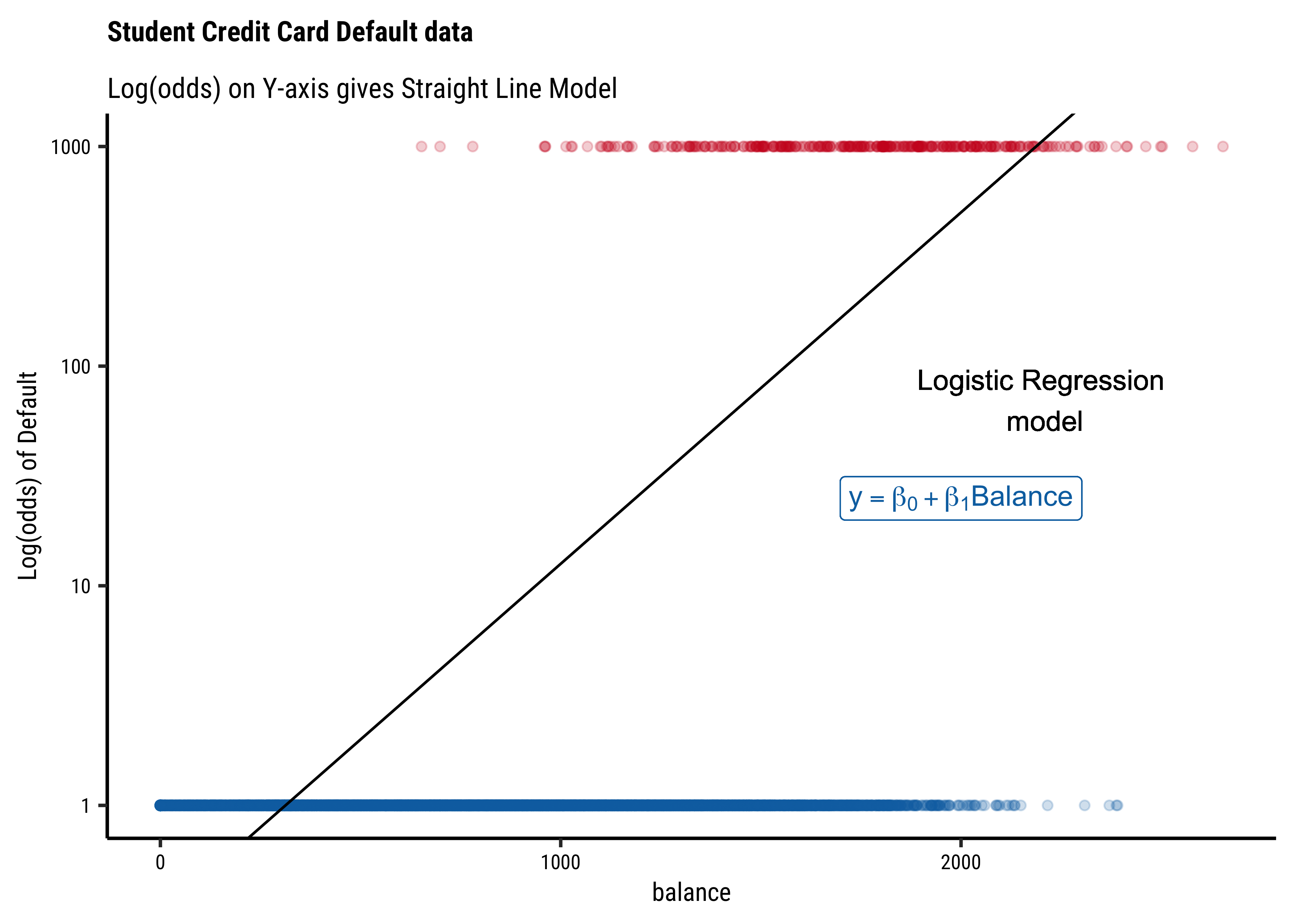
Transformation using
log()?: We need one more leap of faith: how do we convert a
This extends the range of our Qualitative target to the same as with a Quantitative target!
There is an additional benefit if this log() transformation: the Error Distributions with Odds targets. See the plot below. Odds are a necessarily nonlinear function of probability; the slope of Odds ~ probability also depends upon the probability itself, as we saw with the probability curve earlier.
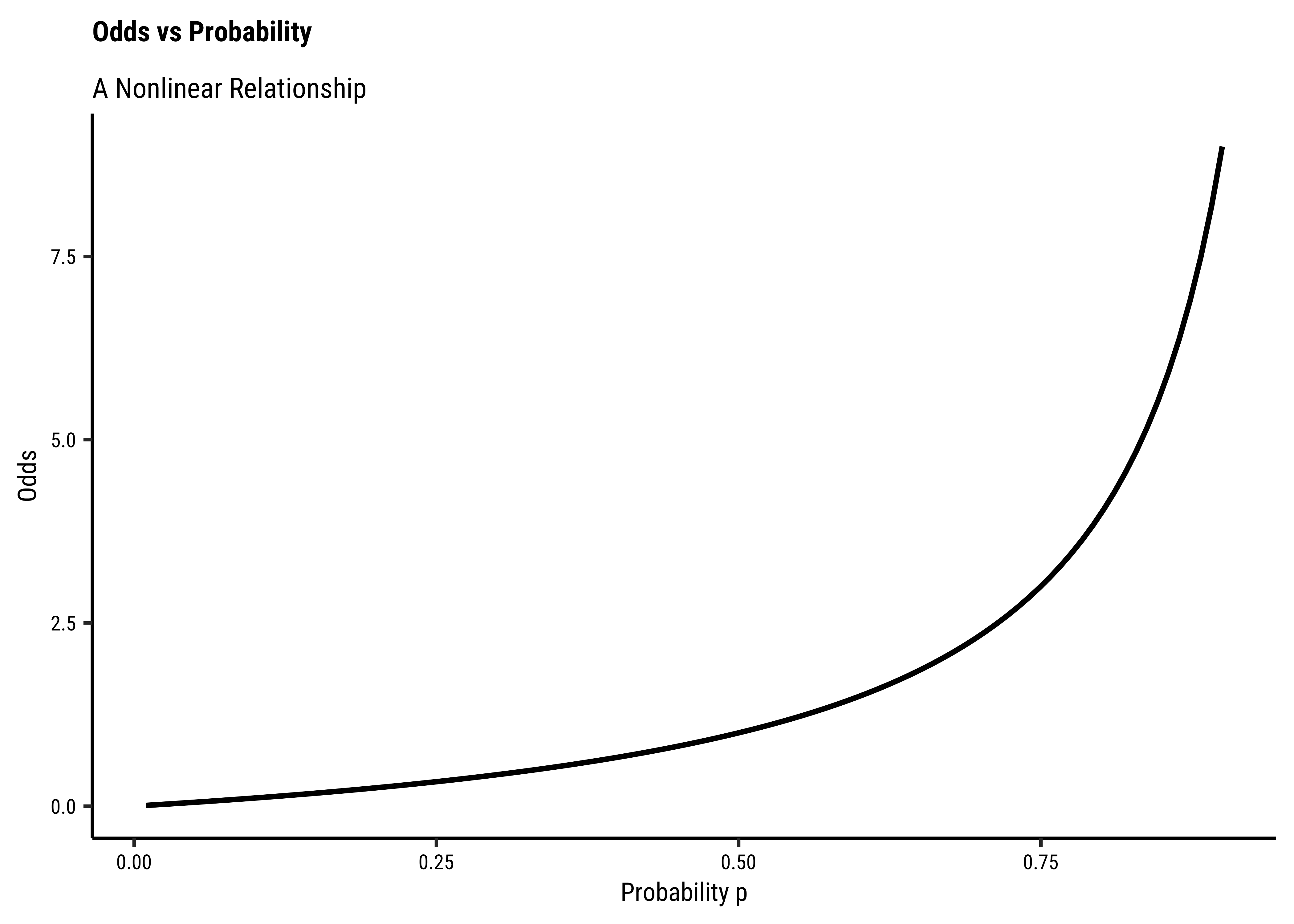
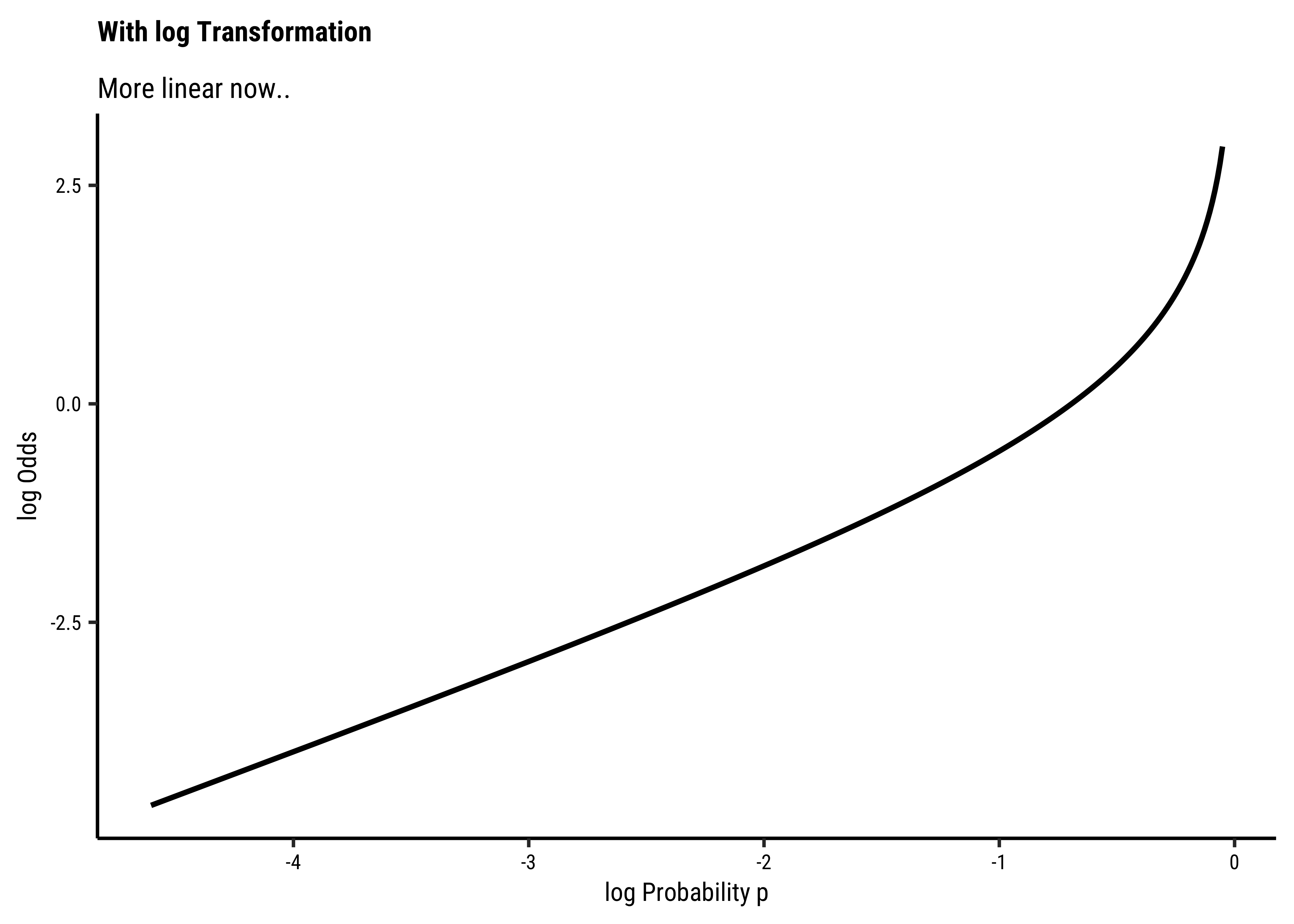
To understand this issue intuitively, consider what happens to, say, a 5% change in the odds ratio near 1.0. If the odds ratio is p and 1-p are log transformation flattens this out to provide a more linear relationship, which is what we desire.
So in our model, instead of modeling odds as the dependent variable, we will use
This is our Logistic Regression Model, which uses a Quantitative Predictor variable to predict a Categorical target variable. We write the model as ( for the Default dataset ) :
This means that:
From the Equation 4 above it should be clear that a unit increase in balance should increase the odds of default by
If we were to include income also as a predictor variable in the model, we might obtain something like:
This model Equation 6 is plotted a little differently, since it includes three variables. We’ll see this shortly, with code. The thing to note is that the formula inside the exp() is a linear combination of the predictors!
-
Estimation of Model Parameters: The parameters
logitsthat we want to model, the logic of minimizing the sum of squared errors(SSE) is no longer appropriate.
The probabilities for default are log(odds) will map respectively to
Instead, we will have to use maximum likelihood estimation(MLE) to estimate the models. The maximum likelihood method maximizes the probability of obtaining the data at hand against every choice of model parameters t and F to evaluate the model comparisons)
Let us proceed with the logistic regression workflow. We will use the well-known Wisconsin breast cancer dataset, readily available from Vincent Arel-Bundock’s website.
cancer <- read_csv("https://vincentarelbundock.github.io/Rdatasets/csv/dslabs/brca.csv") %>%
  janitor::clean_names()
glimpse(cancer)
Rows: 569
Columns: 32
$ rownames <dbl> 1, 2, 3, 4, 5, 6, 7, 8, 9, 10, 11, 12, 13, 14, 15,…
$ x_radius_mean <dbl> 13.540, 13.080, 9.504, 13.030, 8.196, 12.050, 13.4…
$ x_texture_mean <dbl> 14.36, 15.71, 12.44, 18.42, 16.84, 14.63, 22.30, 2…
$ x_perimeter_mean <dbl> 87.46, 85.63, 60.34, 82.61, 51.71, 78.04, 86.91, 7…
$ x_area_mean <dbl> 566.3, 520.0, 273.9, 523.8, 201.9, 449.3, 561.0, 4…
$ x_smoothness_mean <dbl> 0.09779, 0.10750, 0.10240, 0.08983, 0.08600, 0.103…
$ x_compactness_mean <dbl> 0.08129, 0.12700, 0.06492, 0.03766, 0.05943, 0.090…
$ x_concavity_mean <dbl> 0.066640, 0.045680, 0.029560, 0.025620, 0.015880, …
$ x_concave_pts_mean <dbl> 0.047810, 0.031100, 0.020760, 0.029230, 0.005917, …
$ x_symmetry_mean <dbl> 0.1885, 0.1967, 0.1815, 0.1467, 0.1769, 0.1675, 0.…
$ x_fractal_dim_mean <dbl> 0.05766, 0.06811, 0.06905, 0.05863, 0.06503, 0.060…
$ x_radius_se <dbl> 0.2699, 0.1852, 0.2773, 0.1839, 0.1563, 0.2636, 0.…
$ x_texture_se <dbl> 0.7886, 0.7477, 0.9768, 2.3420, 0.9567, 0.7294, 1.…
$ x_perimeter_se <dbl> 2.058, 1.383, 1.909, 1.170, 1.094, 1.848, 1.735, 2…
$ x_area_se <dbl> 23.560, 14.670, 15.700, 14.160, 8.205, 19.870, 20.…
$ x_smoothness_se <dbl> 0.008462, 0.004097, 0.009606, 0.004352, 0.008968, …
$ x_compactness_se <dbl> 0.014600, 0.018980, 0.014320, 0.004899, 0.016460, …
$ x_concavity_se <dbl> 0.023870, 0.016980, 0.019850, 0.013430, 0.015880, …
$ x_concave_pts_se <dbl> 0.013150, 0.006490, 0.014210, 0.011640, 0.005917, …
$ x_symmetry_se <dbl> 0.01980, 0.01678, 0.02027, 0.02671, 0.02574, 0.014…
$ x_fractal_dim_se <dbl> 0.002300, 0.002425, 0.002968, 0.001777, 0.002582, …
$ x_radius_worst <dbl> 15.110, 14.500, 10.230, 13.300, 8.964, 13.760, 15.…
$ x_texture_worst <dbl> 19.26, 20.49, 15.66, 22.81, 21.96, 20.70, 31.82, 2…
$ x_perimeter_worst <dbl> 99.70, 96.09, 65.13, 84.46, 57.26, 89.88, 99.00, 8…
$ x_area_worst <dbl> 711.2, 630.5, 314.9, 545.9, 242.2, 582.6, 698.8, 5…
$ x_smoothness_worst <dbl> 0.14400, 0.13120, 0.13240, 0.09701, 0.12970, 0.149…
$ x_compactness_worst <dbl> 0.17730, 0.27760, 0.11480, 0.04619, 0.13570, 0.215…
$ x_concavity_worst <dbl> 0.239000, 0.189000, 0.088670, 0.048330, 0.068800, …
$ x_concave_pts_worst <dbl> 0.12880, 0.07283, 0.06227, 0.05013, 0.02564, 0.065…
$ x_symmetry_worst <dbl> 0.2977, 0.3184, 0.2450, 0.1987, 0.3105, 0.2747, 0.…
$ x_fractal_dim_worst <dbl> 0.07259, 0.08183, 0.07773, 0.06169, 0.07409, 0.083…
$ y <chr> "B", "B", "B", "B", "B", "B", "B", "B", "B", "B", …skim(cancer)| Name | cancer |
| Number of rows | 569 |
| Number of columns | 32 |
| _______________________ | |
| Column type frequency: | |
| character | 1 |
| numeric | 31 |
| ________________________ | |
| Group variables | None |
Variable type: character
| skim_variable | n_missing | complete_rate | min | max | empty | n_unique | whitespace |
|---|---|---|---|---|---|---|---|
| y | 0 | 1 | 1 | 1 | 0 | 2 | 0 |
Variable type: numeric
| skim_variable | n_missing | complete_rate | mean | sd | p0 | p25 | p50 | p75 | p100 | hist |
|---|---|---|---|---|---|---|---|---|---|---|
| rownames | 0 | 1 | 285.00 | 164.40 | 1.00 | 143.00 | 285.00 | 427.00 | 569.00 | ▇▇▇▇▇ |
| x_radius_mean | 0 | 1 | 14.13 | 3.52 | 6.98 | 11.70 | 13.37 | 15.78 | 28.11 | ▂▇▃▁▁ |
| x_texture_mean | 0 | 1 | 19.29 | 4.30 | 9.71 | 16.17 | 18.84 | 21.80 | 39.28 | ▃▇▃▁▁ |
| x_perimeter_mean | 0 | 1 | 91.97 | 24.30 | 43.79 | 75.17 | 86.24 | 104.10 | 188.50 | ▃▇▃▁▁ |
| x_area_mean | 0 | 1 | 654.89 | 351.91 | 143.50 | 420.30 | 551.10 | 782.70 | 2501.00 | ▇▃▂▁▁ |
| x_smoothness_mean | 0 | 1 | 0.10 | 0.01 | 0.05 | 0.09 | 0.10 | 0.11 | 0.16 | ▁▇▇▁▁ |
| x_compactness_mean | 0 | 1 | 0.10 | 0.05 | 0.02 | 0.06 | 0.09 | 0.13 | 0.35 | ▇▇▂▁▁ |
| x_concavity_mean | 0 | 1 | 0.09 | 0.08 | 0.00 | 0.03 | 0.06 | 0.13 | 0.43 | ▇▃▂▁▁ |
| x_concave_pts_mean | 0 | 1 | 0.05 | 0.04 | 0.00 | 0.02 | 0.03 | 0.07 | 0.20 | ▇▃▂▁▁ |
| x_symmetry_mean | 0 | 1 | 0.18 | 0.03 | 0.11 | 0.16 | 0.18 | 0.20 | 0.30 | ▁▇▅▁▁ |
| x_fractal_dim_mean | 0 | 1 | 0.06 | 0.01 | 0.05 | 0.06 | 0.06 | 0.07 | 0.10 | ▆▇▂▁▁ |
| x_radius_se | 0 | 1 | 0.41 | 0.28 | 0.11 | 0.23 | 0.32 | 0.48 | 2.87 | ▇▁▁▁▁ |
| x_texture_se | 0 | 1 | 1.22 | 0.55 | 0.36 | 0.83 | 1.11 | 1.47 | 4.88 | ▇▅▁▁▁ |
| x_perimeter_se | 0 | 1 | 2.87 | 2.02 | 0.76 | 1.61 | 2.29 | 3.36 | 21.98 | ▇▁▁▁▁ |
| x_area_se | 0 | 1 | 40.34 | 45.49 | 6.80 | 17.85 | 24.53 | 45.19 | 542.20 | ▇▁▁▁▁ |
| x_smoothness_se | 0 | 1 | 0.01 | 0.00 | 0.00 | 0.01 | 0.01 | 0.01 | 0.03 | ▇▃▁▁▁ |
| x_compactness_se | 0 | 1 | 0.03 | 0.02 | 0.00 | 0.01 | 0.02 | 0.03 | 0.14 | ▇▃▁▁▁ |
| x_concavity_se | 0 | 1 | 0.03 | 0.03 | 0.00 | 0.02 | 0.03 | 0.04 | 0.40 | ▇▁▁▁▁ |
| x_concave_pts_se | 0 | 1 | 0.01 | 0.01 | 0.00 | 0.01 | 0.01 | 0.01 | 0.05 | ▇▇▁▁▁ |
| x_symmetry_se | 0 | 1 | 0.02 | 0.01 | 0.01 | 0.02 | 0.02 | 0.02 | 0.08 | ▇▃▁▁▁ |
| x_fractal_dim_se | 0 | 1 | 0.00 | 0.00 | 0.00 | 0.00 | 0.00 | 0.00 | 0.03 | ▇▁▁▁▁ |
| x_radius_worst | 0 | 1 | 16.27 | 4.83 | 7.93 | 13.01 | 14.97 | 18.79 | 36.04 | ▆▇▃▁▁ |
| x_texture_worst | 0 | 1 | 25.68 | 6.15 | 12.02 | 21.08 | 25.41 | 29.72 | 49.54 | ▃▇▆▁▁ |
| x_perimeter_worst | 0 | 1 | 107.26 | 33.60 | 50.41 | 84.11 | 97.66 | 125.40 | 251.20 | ▇▇▃▁▁ |
| x_area_worst | 0 | 1 | 880.58 | 569.36 | 185.20 | 515.30 | 686.50 | 1084.00 | 4254.00 | ▇▂▁▁▁ |
| x_smoothness_worst | 0 | 1 | 0.13 | 0.02 | 0.07 | 0.12 | 0.13 | 0.15 | 0.22 | ▂▇▇▂▁ |
| x_compactness_worst | 0 | 1 | 0.25 | 0.16 | 0.03 | 0.15 | 0.21 | 0.34 | 1.06 | ▇▅▁▁▁ |
| x_concavity_worst | 0 | 1 | 0.27 | 0.21 | 0.00 | 0.11 | 0.23 | 0.38 | 1.25 | ▇▅▂▁▁ |
| x_concave_pts_worst | 0 | 1 | 0.11 | 0.07 | 0.00 | 0.06 | 0.10 | 0.16 | 0.29 | ▅▇▅▃▁ |
| x_symmetry_worst | 0 | 1 | 0.29 | 0.06 | 0.16 | 0.25 | 0.28 | 0.32 | 0.66 | ▅▇▁▁▁ |
| x_fractal_dim_worst | 0 | 1 | 0.08 | 0.02 | 0.06 | 0.07 | 0.08 | 0.09 | 0.21 | ▇▃▁▁▁ |
We see that there are 31 Quantitative variables, all named as x_***, and one Qualitative variable,y, which is a two-level target. (B = Benign, M = Malignant). The dataset has 569 observations, and no missing data.
Let us rename y as diagnosis and take two other Quantitative parameters as predictors, suitably naming them too. We will also create a binary-valued variable called diagnosis_malignant (Binary, Malignant = 1, Benign = 0) for use as a target in our logistic regression model.
Show the Code
cancer_modified <- cancer %>%
  rename(
    "diagnosis" = y,
    "radius_mean" = x_radius_mean,
    "concave_points_mean" = x_concave_pts_mean
  ) %>%
  ## Convert diagnosis to factor
  mutate(diagnosis = factor(
    diagnosis,
    levels = c("B", "M"),
    labels = c("B", "M")
  )) %>%
  ## New Variable
  mutate(diagnosis_malignant = if_else(diagnosis == "M", 1, 0)) %>%
  select(radius_mean, concave_points_mean, diagnosis, diagnosis_malignant)

cancer_modifiedradius_mean <dbl> | concave_points_mean <dbl> | diagnosis <fct> | diagnosis_malignant <dbl> | |
|---|---|---|---|---|
| 13.540 | 0.047810 | B | 0 | |
| 13.080 | 0.031100 | B | 0 | |
| 9.504 | 0.020760 | B | 0 | |
| 13.030 | 0.029230 | B | 0 | |
| 8.196 | 0.005917 | B | 0 | |
| 12.050 | 0.027490 | B | 0 | |
| 13.490 | 0.033840 | B | 0 | |
| 11.760 | 0.011150 | B | 0 | |
| 13.640 | 0.017230 | B | 0 | |
| 11.940 | 0.013490 | B | 0 |
How can we predict whether a cancerous tumour is Benign or Malignant, based on the variable radius_mean alone, and with both radius_mean and concave_points_mean?
Let us use GGally to plot a set of combo-plots for our modified dataset:
Show the Code
theme_set(new = theme_custom())
#
cancer_modified %>%
  select(diagnosis, radius_mean, concave_points_mean) %>%
  GGally::ggpairs(
    mapping = aes(colour = diagnosis),
    switch = "both",
    # axis labels in more traditional locations(left and bottom)

    progress = FALSE,
    # no compute progress messages needed

    # Choose the diagonal graphs (always single variable! Think!)
    diag = list(continuous = "densityDiag", alpha = 0.3),
    # choosing density

    # Choose lower triangle graphs, two-variable graphs
    lower = list(continuous = wrap("points", alpha = 0.3)),
    title = "Cancer Pairs Plot #1"
  ) +
  scale_color_brewer(
    palette = "Set1",
    aesthetics = c("color", "fill")
  )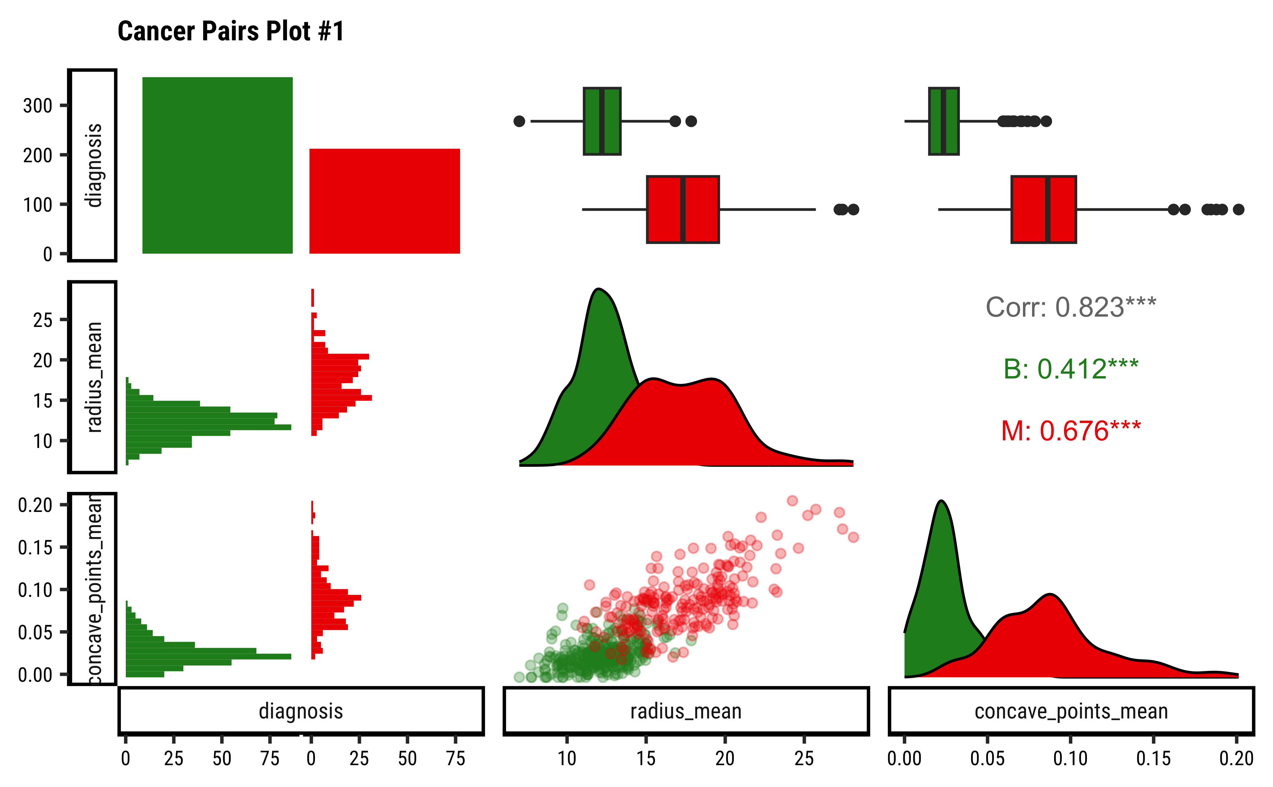
- The counts for “B” and “M” are not terribly unbalanced; and both the
radius_meanandconcave_pts_meanappear to have well-separated box plot distributions for “B” and “M”. - Given the visible separation of the box-plots for both variables
radius_meanandconcave_pts_mean, we can believe that these will be good choices as predictors. - Interestingly,
radius_meanandconcave_pts_meanare also mutually well-correlated, with a
Let us code two models, using one and then both the predictor variables:
Show the Code
The equation for the simple model is:
Increasing radius_mean by one unit changes the log odds by
Show the Code
# Set graph theme
theme_set(new = theme_custom())
##
qthresh <- c(0.2, 0.5, 0.8)
beta01 <- coef(cancer_fit_1)[1]
beta11 <- coef(cancer_fit_1)[2]
decision_point <- (log(qthresh / (1 - qthresh)) - beta01) / beta11
##
cancer_modified %>%
  gf_point(
    diagnosis_malignant ~ radius_mean,
    colour = ~diagnosis,
    title = "diagnosis ~ radius_mean",
    xlab = "Average radius",
    ylab = "Diagnosis (1=malignant)", size = 3, show.legend = F
  ) %>%
  # gf_fun(exp(1.033 * radius_mean - 15.25) / (1 + exp(1.033 * radius_mean - 15.25)) ~ radius_mean, xlim = c(1, 30), linewidth = 3, colour = "red") %>%
  gf_smooth(
    method = glm,
    method.args = list(family = "binomial"),
    se = FALSE,
    color = "black"
  ) %>%
  gf_vline(xintercept = decision_point, linetype = "dashed") %>%
  gf_refine(annotate(
    "text",
    label = paste0("q = ", qthresh),
    x = decision_point + 0.45,
    y = 0.4,
    angle = -90
  ), scale_color_brewer(palette = "Set1")) %>%
  gf_hline(yintercept = 0.5) %>%
  gf_theme(theme(plot.title.position = "plot")) %>%
  gf_refine(xlim(5, 30))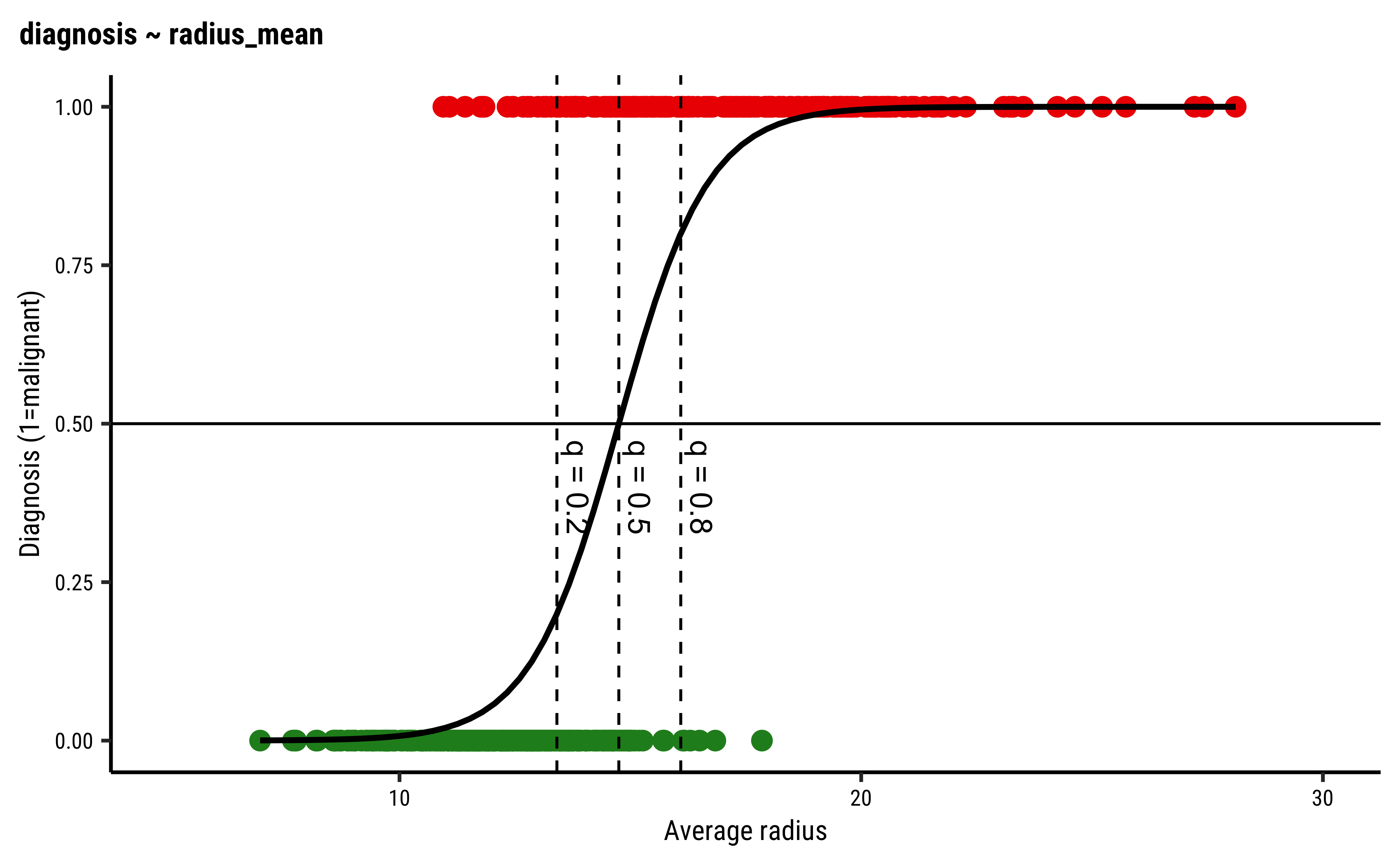
The dotted lines show how the model can be used to classify the data in to two classes (“B” and “M”) depending upon the threshold probability
Taking both predictor variables, we obtain the model:
Show the Code
The equation for the more complex model is:
Increasing radius_mean by one unit changes the log odds by concave_points_mean is held fixed.
We can plot the model as shown below: we create a scatter plot of the two predictor variables. The superimposed diagonal lines are lines for several constant values of threshold probability
Show the Code
# Set graph theme
theme_set(new = theme_custom())
##
beta02 <- coef(cancer_fit_2)[1]
beta12 <- coef(cancer_fit_2)[2]
beta22 <- coef(cancer_fit_2)[3]
##
decision_intercept <- 1 / beta22 * (log(qthresh / (1 - qthresh)) - beta02)
decision_slope <- -beta12 / beta22
##
cancer_modified %>%
  gf_point(concave_points_mean ~ radius_mean,
    color = ~diagnosis, shape = ~diagnosis,
    size = 3, alpha = 0.5
  ) %>%
  gf_labs(
    x = "Average radius",
    y = "Average concave\nportions of the\ncontours",
    color = "Diagnosis",
    shape = "Diagnosis",
    title = "diagnosis ~ radius_mean + concave_points_mean"
  ) %>%
  gf_abline(
    slope = decision_slope, intercept = decision_intercept,
    linetype = "dashed"
  ) %>%
  gf_refine(
    scale_color_brewer(palette = "Set1"),
    annotate("text", label = paste0("q = ", qthresh), x = 10, y = c(0.08, 0.1, 0.115), angle = -17.155)
  ) %>%
  gf_theme(theme(plot.title.position = "plot"))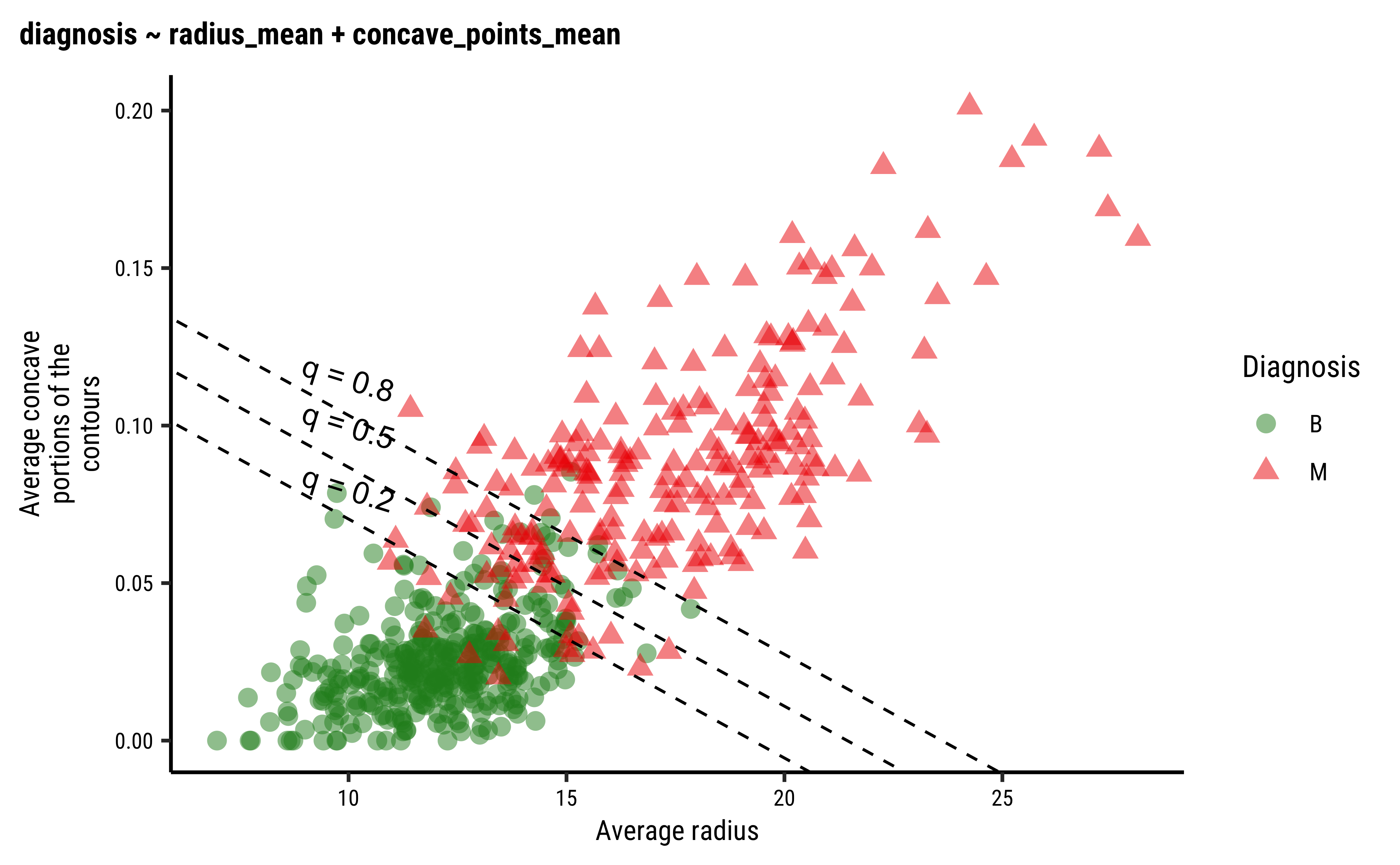
To Be Written Up.
To Be Written Up.
To Be Written Up.
Workflow: Logistic Regression Internals
All that is very well, but what is happening under the hood of the glm command? Consider the diagnosis (target) variable and say the average_radius feature/predictor variable. What we do is:
- Plot a scatter plot
gf_point(diagnosis ~ average_radius, data = cancer_modified) - Start with a sigmoid curve with some initial parameters
diagnosisfor any givenaverage_radius - We know the target labels for each data point ( i.e. “B” and “M”). We can calculate the likelihood of
- We then change the values of
- The set of parameters with the maximum likelihood(ML) for
- Use that model henceforth as a model for prediction.
How does one find out the “ML” parameters? There is clearly a two step procedure:
- Find the likelihood of the data for the parameters
- Maximize the likelihood by varying them. In practice, the changes to the parameters (step 5) are made in accordance with a method such as the Newton-Raphson method that can rapidly find the ML values for the parameters.
Let us visualize the variations and computations from step(5). For the sake of clarity:
- we will take a small sample of the original dataset
- we take several different values for
- Use these get a set of regression curves
- which we superimpose on the scatter plot of the sample
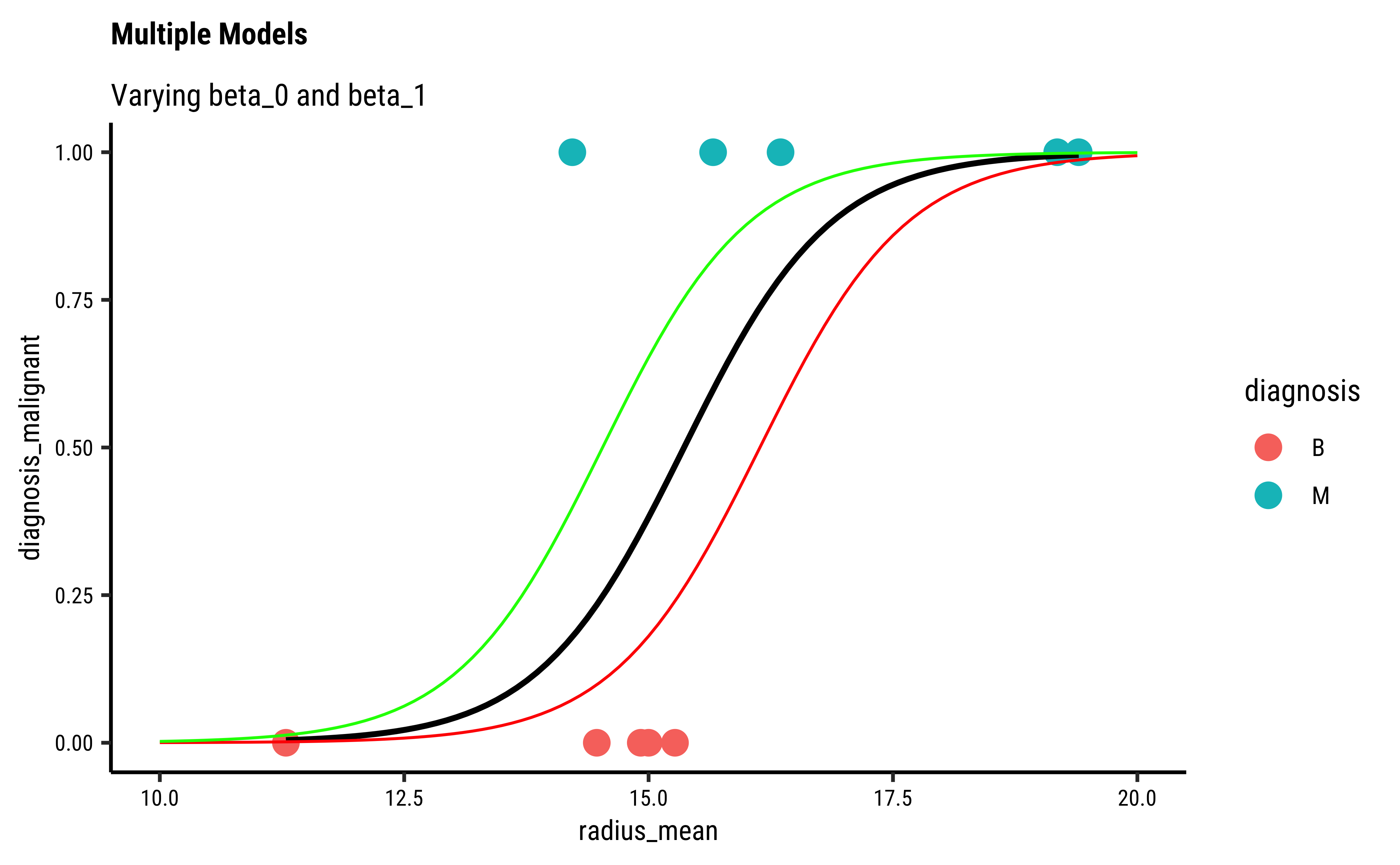
In Figure 6, we see three models: the “optimum” one in black, and two others in green and orange respectively.
We now project the actual points on to the regression curve, to obtain the predicted probability for each point.
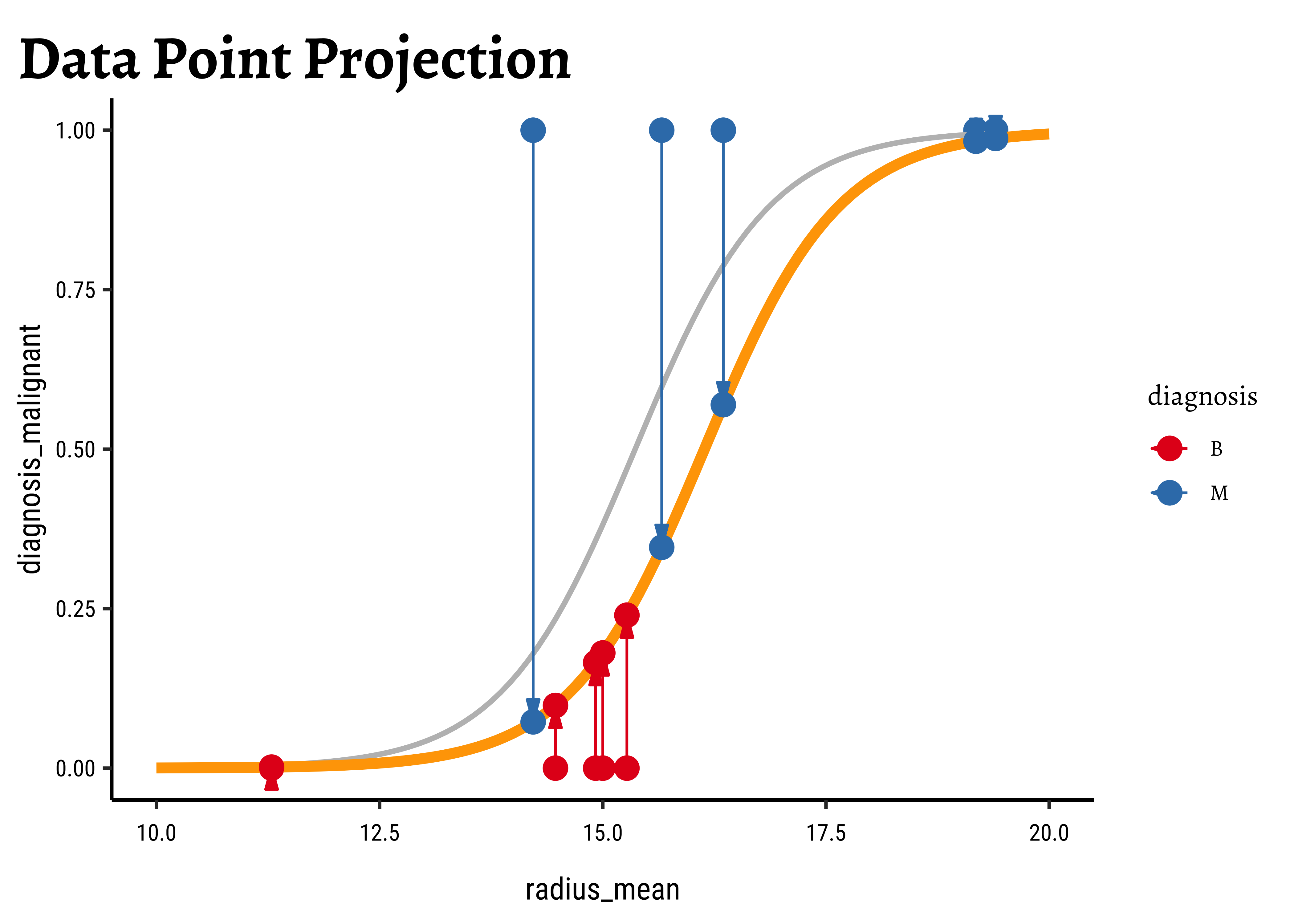
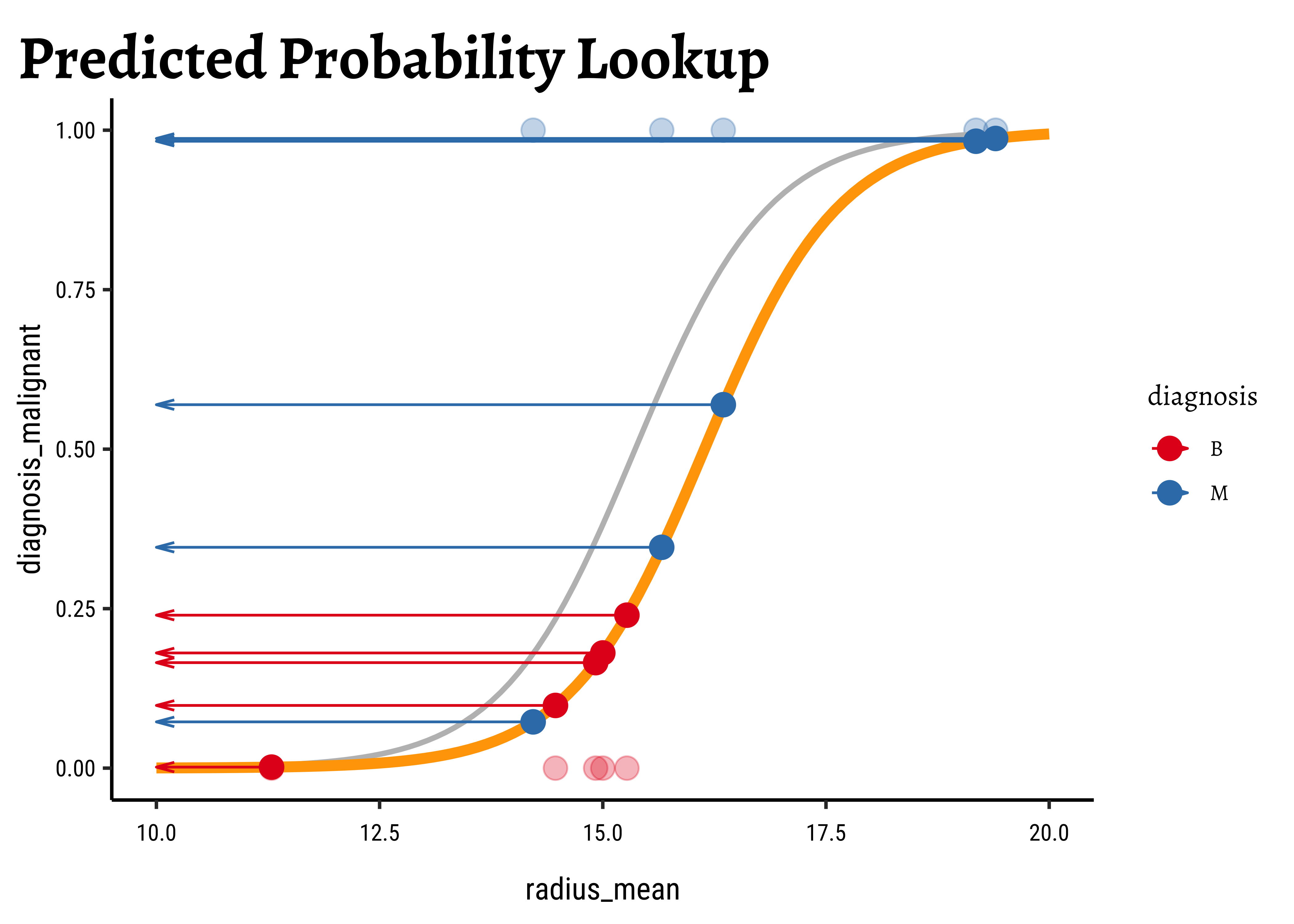
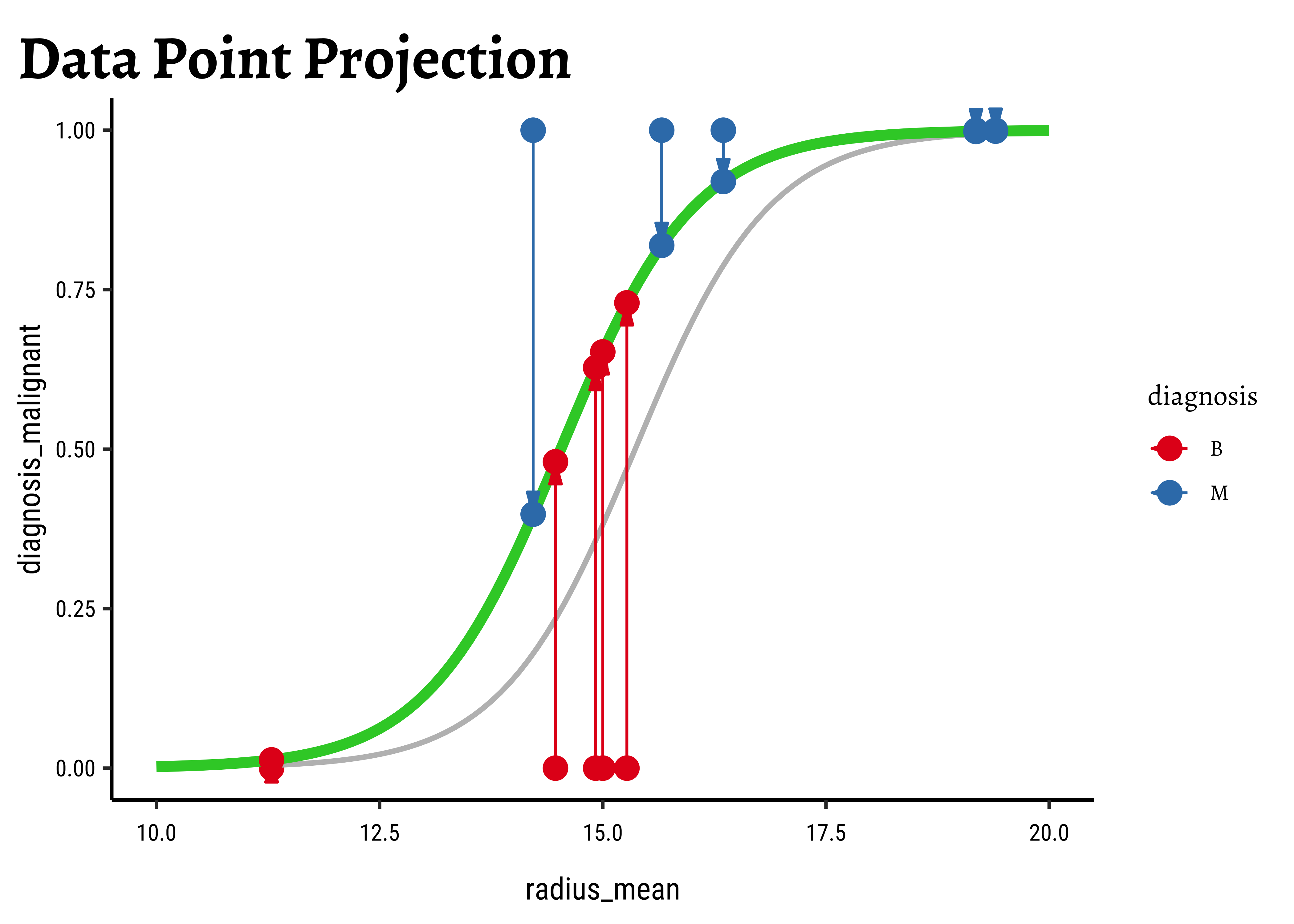
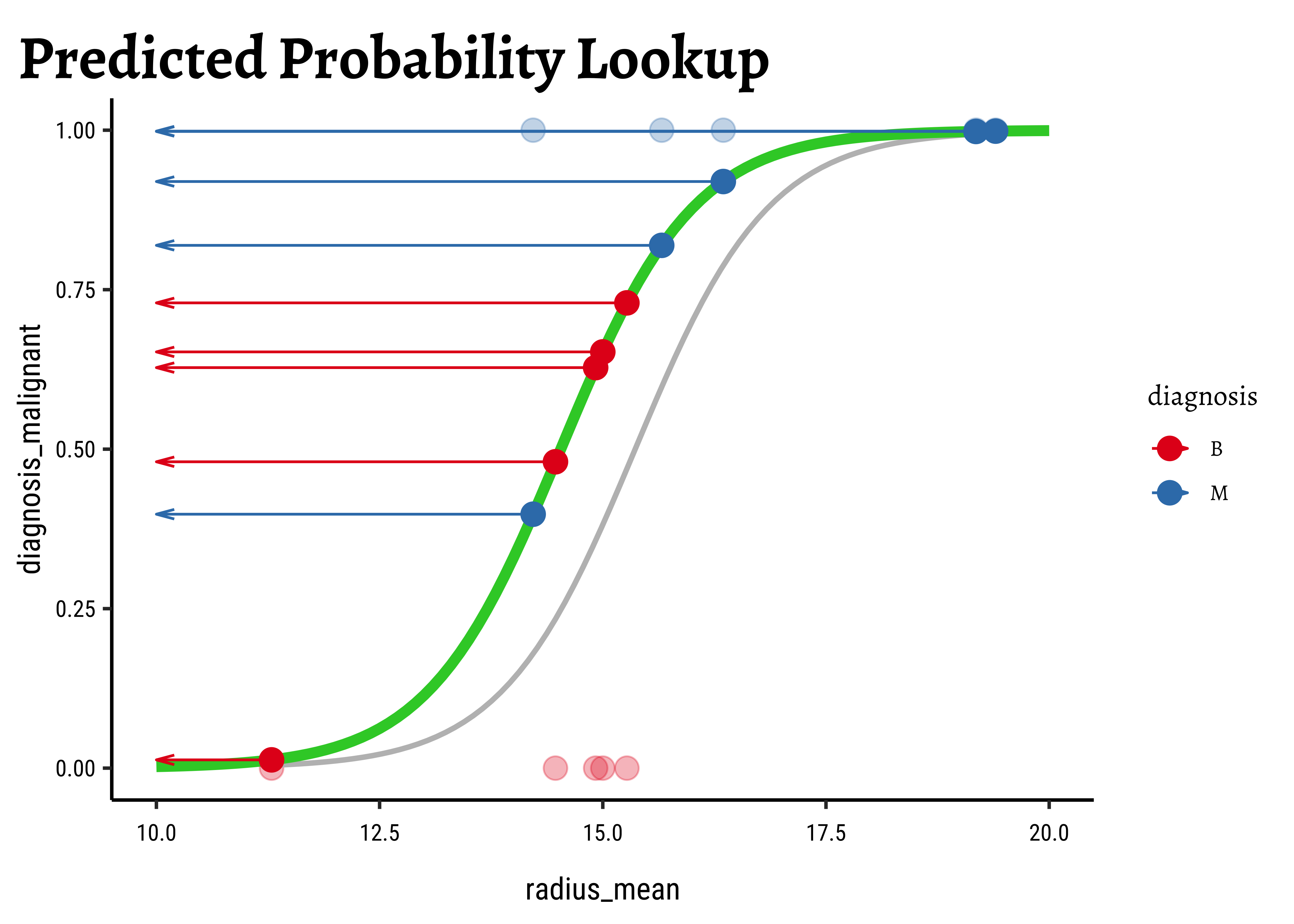
The predicted probability
We now need to find the (global) maximum of this quantity and determine the
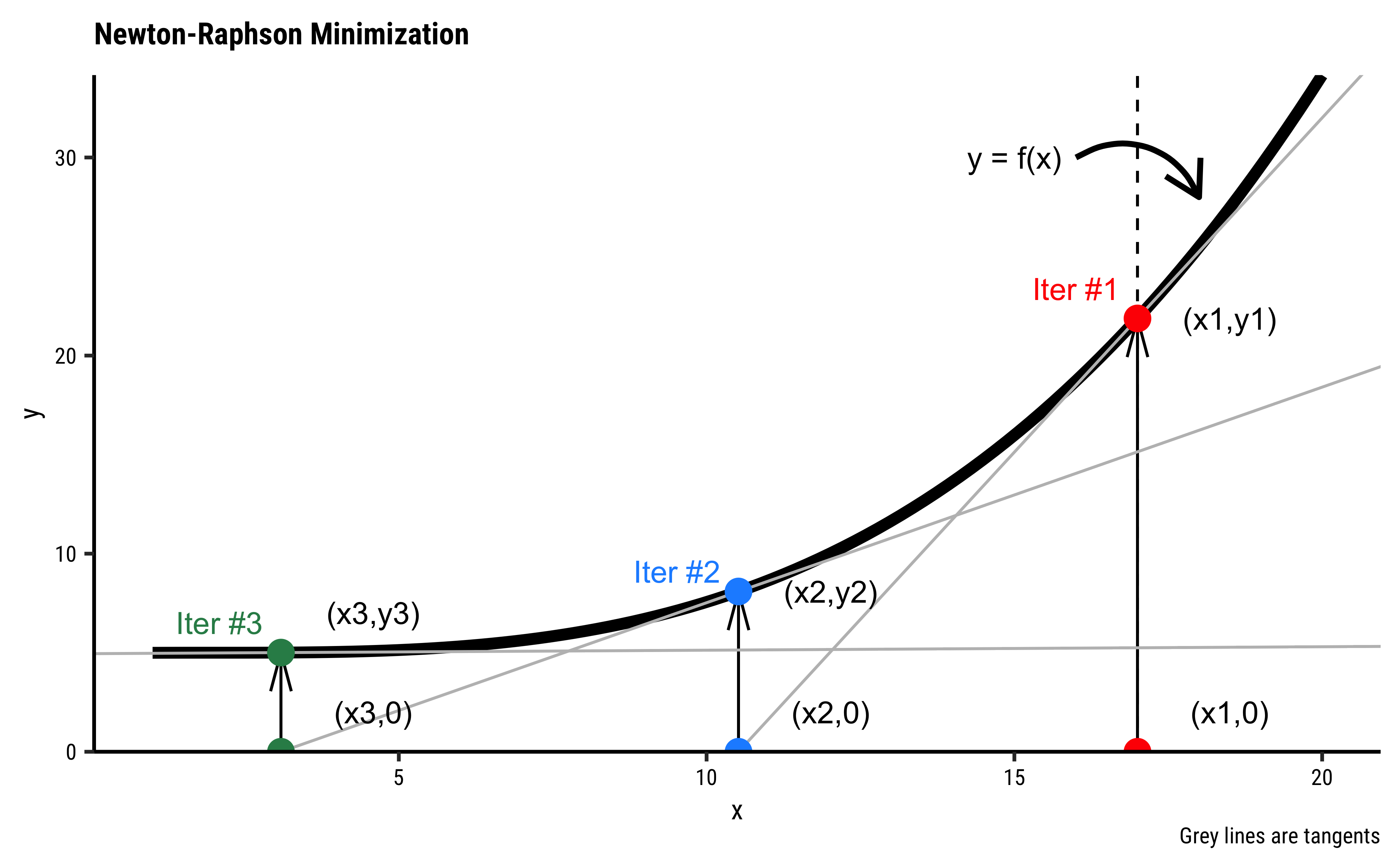
- The black curve
- We start with any arbitrary starting value of
- The tangent
- Repeat.
- Stop when the gradient becomes very small and
How do we calculate the next value of x using the tangent?
- At
- This equation applies at point
- Solving for
- Since
To be written up:
- Formula for gradient of LL
- Convergence of Newton- Raphson method for Maximum Likelihood
- Hand Calculation of all steps (!!)
- Logistic Regression is a great ML algorithm for predicting Qualitative target variables.
- It also works for multi-level/multi-valued Qual variables (multinomial logistic regression)
- The internals of Logistic Regression are quite different compared to Linear Regression
- Judd, Charles M. & McClelland, Gary H. & Ryan, Carey S. Data Analysis: A Model Comparison Approach to Regression, ANOVA, and Beyond. Routledge, Aug 2017. Chapter 14.
- Emi Tanaka.Logistic Regression https://emitanaka.org/iml/lectures/lecture-04A.html#/TOC. Course: ETC3250/5250, Monash University, Melbourne, Australia.
- Geeks for Geeks.Logistic Regression. https://www.geeksforgeeks.org/understanding-logistic-regression/
- Geeks for Geeks.Maximum Likelihood Estimation. https://www.geeksforgeeks.org/probability-density-estimation-maximum-likelihood-estimation/
- https://yury-zablotski.netlify.app/post/how-logistic-regression-works/
- https://uc-r.github.io/logistic_regression
- https://francisbach.com/self-concordant-analysis-for-logistic-regression/
- https://statmath.wu.ac.at/courses/heather_turner/glmCourse_001.pdf
- https://jasp-stats.org/2022/06/30/generalized-linear-models-glm-in-jasp/
- P. Bingham, N.Q. Verlander, M.J. Cheal (2004). John Snow, William Farr and the 1849 outbreak of cholera that affected London: a reworking of the data highlights the importance of the water supply. Public Health Volume 118, Issue 6, September 2004, Pages 387-394. Read the PDF.
- https://peopleanalytics-regression-book.org/bin-log-reg.html
- McGill University. Epidemiology https://www.medicine.mcgill.ca/epidemiology/joseph/courses/epib-621/logfit.pdf
- https://arunaddagatla.medium.com/maximum-likelihood-estimation-in-logistic-regression-f86ff1627b67
Footnotes
Citation
@online{v.2023,
  author = {V., Arvind},
  title = {Modelling with {Logistic} {Regression}},
  date = {2023-04-13},
  url = {https://av-quarto.netlify.app/content/courses/Analytics/Modelling/Modules/LogReg/},
  langid = {en},
  abstract = {Predicting Qualitative Target Variables}
}