Euler Formula
Parametric Equations
Rotation
Symmetry
Introduction
Let us start with an investigation into rolling circles! Circles have been with us since our childhood toys and to our older (and more silly!) aspirations for wheels (ahem!). Let us understand their mathematics and see what we can make with them.

What is a Parametric Equation?
How was this curve created? The equation for the curve is given by a pair of parametric equations, one for
This form is especially suited for a computational depiction of the curve, since we can have the parameter
How about the Euler Formula?
What is the equation of a circle? Most likely you will say:
for a circle with center
As Frank Farris says, this is fine, but it represents a static view of a circle, which is not the simplest way to direct the drawing of one. The simplest way to instruct a machine to draw a circle uses a parametric form discussed above, also known as a vector-valued function:
Now, if we were to use complex numbers as our notation, then the function for our circle becomes:
where of course,
This is the famous Euler Formula that connects complex numbers with trigonometry.
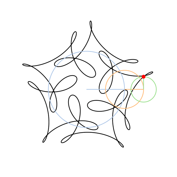
The Mystery Curve
Using this formula, our parametric function
and
which gives us three rotating vectors with amplitudes given by {1, 1/2, 1/3} and with rotation speeds in the ratio {1 : 6: -14}. The first two rotate counter-clockwise; the third vector rotates in the clockwise direction since we have a negative coefficient for
How do we go from the parametric form in Equation 1 to the complex exponential form in Equation 4? The first two terms are direct combinings of the respective cos and sin terms into exponentials; the third term may need a bit of understanding.
Here the
which are respectively the desired x and y parametric functions for the third term.
Reverse Rotating Vectors and Complex Amplitudes!!
Sigh.
| Amplitude | Rotation | Example | Operation in Parametric Equation | What does it mean, really? |
|---|---|---|---|---|
| Real | Positive/CCW |
|
Vector starts from x-axis, goes CCW | |
| Real | Negative/CW |
|
Vector starts from x-axis, goes CW | |
| Complex | Positive/CCW |
|
Vector starts at |
|
| Complex | Negative/CW |
|
Vector starts at |
Do think of what might happen when the amplitude has an overall negative sign, like
Plotting with Complex Exponentials in R
We can use the rules in the above table to directly plot using complex vectors in R:
Show the Code
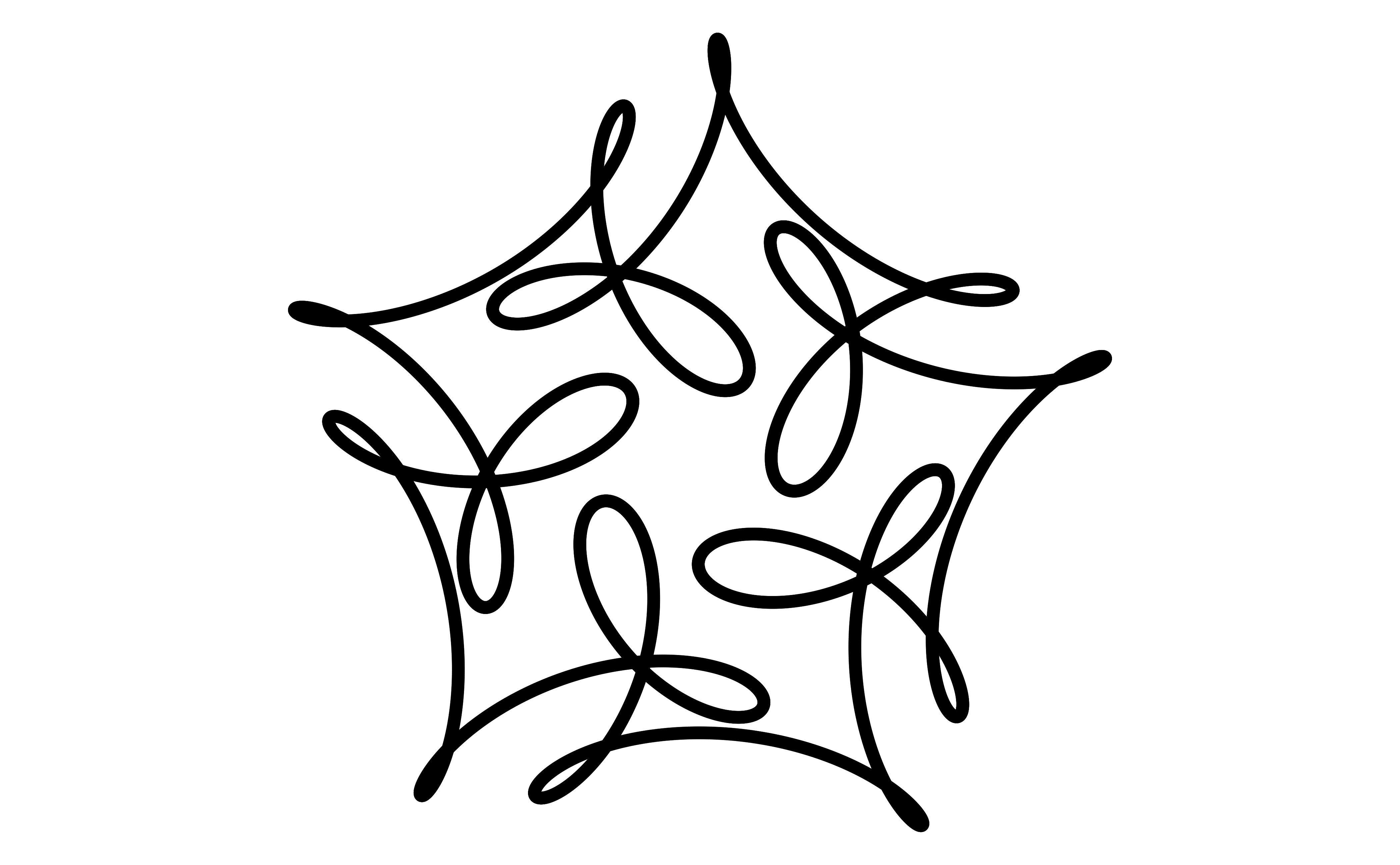
Rotational Symmetry
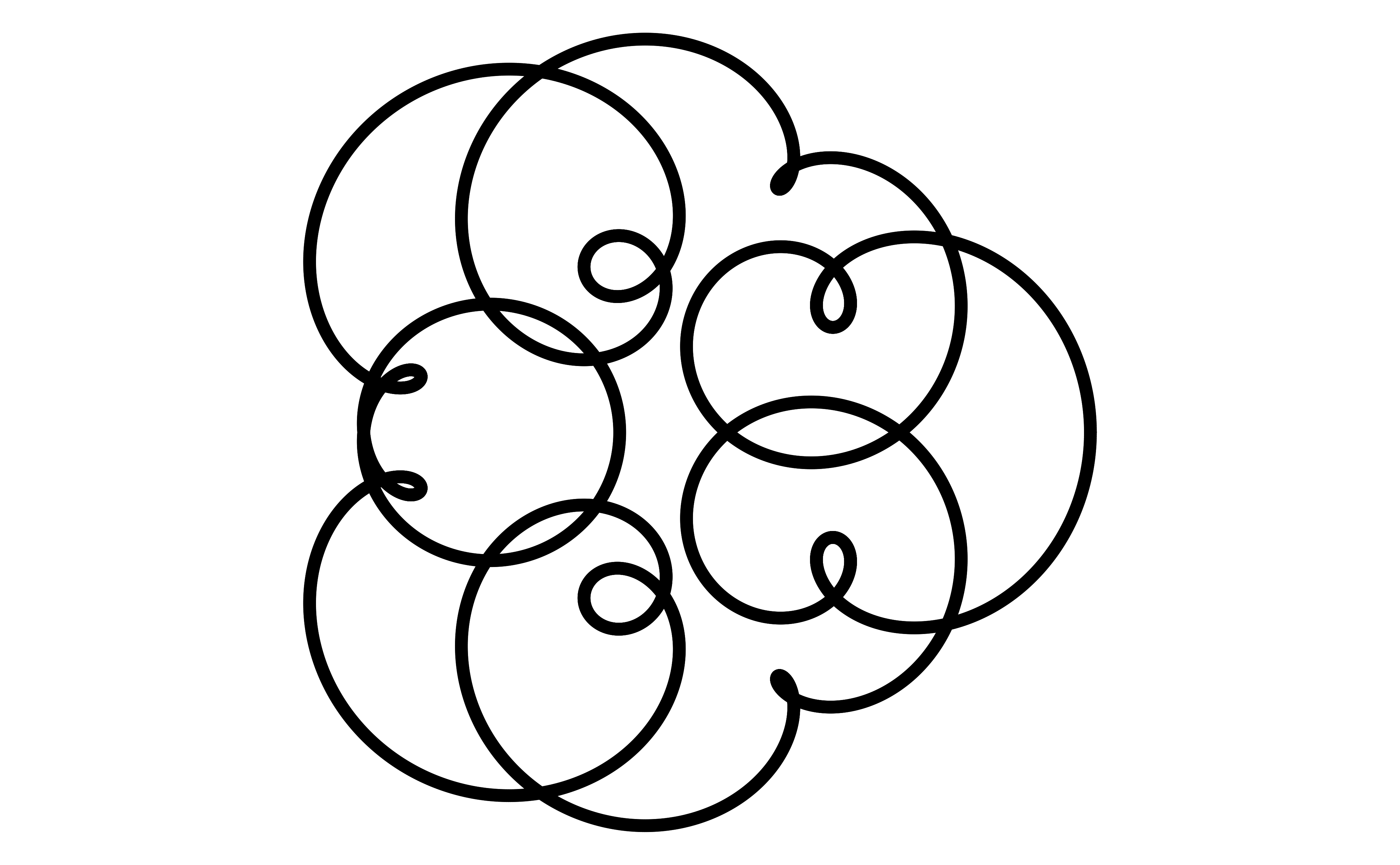
We notice a pattern in Figure 1, our inspiration example: the shape has a five-fold symmetry: If we rotate the entire figure by
Following the development in Frank Farris’ book, let us record our ideas/suspicions of symmetry as:
Does this work out? Let’s see:
So if we shift time by
Time shifts are Angle Shifts. And our mystery curve hence meets the symmetry condition in Equation 5.
The Symmetry Condition Theorem
Suppose that
Then, for any choice of the complex coefficients
What a mouthful! What does that mean?
If we take a set of
Complex Coefficients?
Question: How do we handle
Look back at the table Table 1.
Consider a
We can view this as a rotation by
Mutually Prime?
Question: What happens when
Design Principles for Rotational Symmetry
How do we capture all of the above in a set of design principles for symmetric rotation-based patterns? The design parameters for us are:
- Number of frequencies / rolling circles: M
- The Frequency values for each rolling circle:
- The (complex) Amplitudes
Larger values of
Let us randomly create an equation, using the following parameters:
- M = 5 (Number of rotating circles)
- m = 7 (Prime Modulus) i.e. Order of Symmetry
- k = 2 (The remainder of
Here is the plot of the frequency components:
Show the Code
# Set graph theme
theme_set(new = theme_custom())
#
set.seed(42)
M <- 5 # Number of circles
m <- 7 # Prime Modulus
k <- 2 # Type of Symmetry
tibble(
  index = seq(-floor((M - 1) / 2), floor((M - 1) / 2), 1),
  prime_multiple = m * index,
  remainder = rep(k, length(index)),
  frequency = prime_multiple + remainder
) %>%
  mutate(amplitude = if_else(frequency == k, 1, k / frequency)) %>%
  # scaling amplitudes
  # mutate(y0 = rep(0, length(index)),
  #        z0 = rep(0, length(index))) %>%
  dplyr::select(prime_multiple, frequency, amplitude) -> circles
circlesprime_multiple <dbl> | frequency <dbl> | amplitude <dbl> | ||
|---|---|---|---|---|
| -14 | -12 | -0.1666667 | ||
| -7 | -5 | -0.4000000 | ||
| 0 | 2 | 1.0000000 | ||
| 7 | 9 | 0.2222222 | ||
| 14 | 16 | 0.1250000 |
Show the Code
##
circles %>%
  gf_hline(yintercept = 0, colour = "grey") %>%
  gf_segment(rep(0, length(prime_multiple)) + rep(0, length(prime_multiple)) ~ prime_multiple + frequency,
    arrow = arrow(
      angle = 20,
      length = unit(0.15, "inches"),
      ends = "last", type = "open"
    )
  ) %>%
  gf_segment(
    rep(0, length(prime_multiple)) + amplitude ~
      frequency + frequency,
    data = circles, linewidth = 2,
    arrow = arrow(
      angle = 30,
      length = unit(0.1, "inches"),
      ends = "last", type = "open"
    )
  ) %>%
  gf_point(rep(0, length(prime_multiple)) ~ prime_multiple,
    colour = "red", size = 3
  ) %>%
  gf_point(rep(0, length(prime_multiple)) ~ frequency,
    xlab = "Frequency Component",
    ylab = "Amplitude", data = circles
  ) %>%
  gf_labs(
    title = "Rotating Vectors Frquencies and Amplitudes",
    subtitle = "Negative Frequency components rotate counterclockwise", caption = "Red Dots: Prime Modulus Multiples"
  ) %>%
  gf_refine(annotate(
    x = circles$frequency + 1.75,
    y = circles$amplitude,
    geom = "text",
    label = as.character(round(circles$amplitude, 4), nsmall = 3), size = 3.5
  )) %>%
  gf_refine(scale_x_continuous(breaks = c(-28, -21, -14, -7, -5, 0, 2, 7, 9, 14, 16))) %>%
  gf_theme(theme_custom())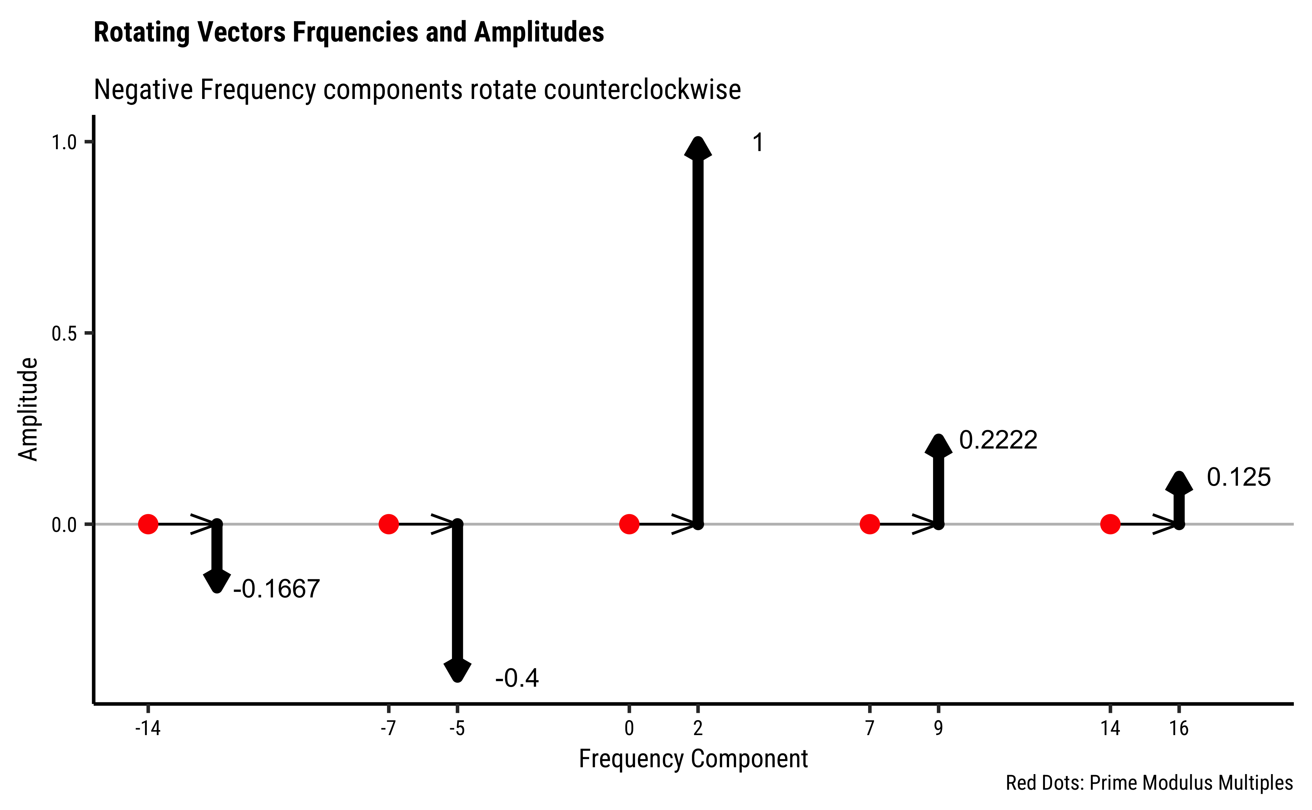
The function for this curve would be:
Let us now plot this:
Show the Code
# remainder = 2 from 7
# frequencies: 2, 7+2, 14+2, -7+2, -14+2
f_mystery2 <- function(x) {
  1.0 * (exp((0 + 2i) * x) +
    0.2222 * exp((0 + 9i) * x) +
    0.125 * exp((0 + 16i) * x) -
    0.4 * exp((0 - 5i) * x) -
    0.1667 * exp((0 - 12i) * x))
}
data_mystery_2 <- tibble(t, pattern = f_mystery2(t))
data_mystery_2 %>%
  gf_point(Im(pattern) ~ Re(pattern), title = "Complex Exponential Rendering
           ") %>%
  gf_refine(coord_equal()) %>%
  gf_theme(theme_void())
###
data2 <- tibble::tibble(
  t = seq(0, 2 * pi, 0.001),
  x = cos(2 * t) + 0.2222 * cos(9 * t) + 0.125 * cos(16 * t) - 0.4 * cos(5 * t) - 0.1667 * cos(12 * t),
  y = sin(2 * t) + 0.2222 * sin(9 * t) + 0.125 * sin(16 * t) + 0.4 * sin(5 * t) + 0.1667 * sin(12 * t)
)
data2 %>%
  gf_point(y ~ x, title = "Parametric Equation Rendering") %>%
  gf_refine(coord_equal()) %>%
  gf_theme(theme_void())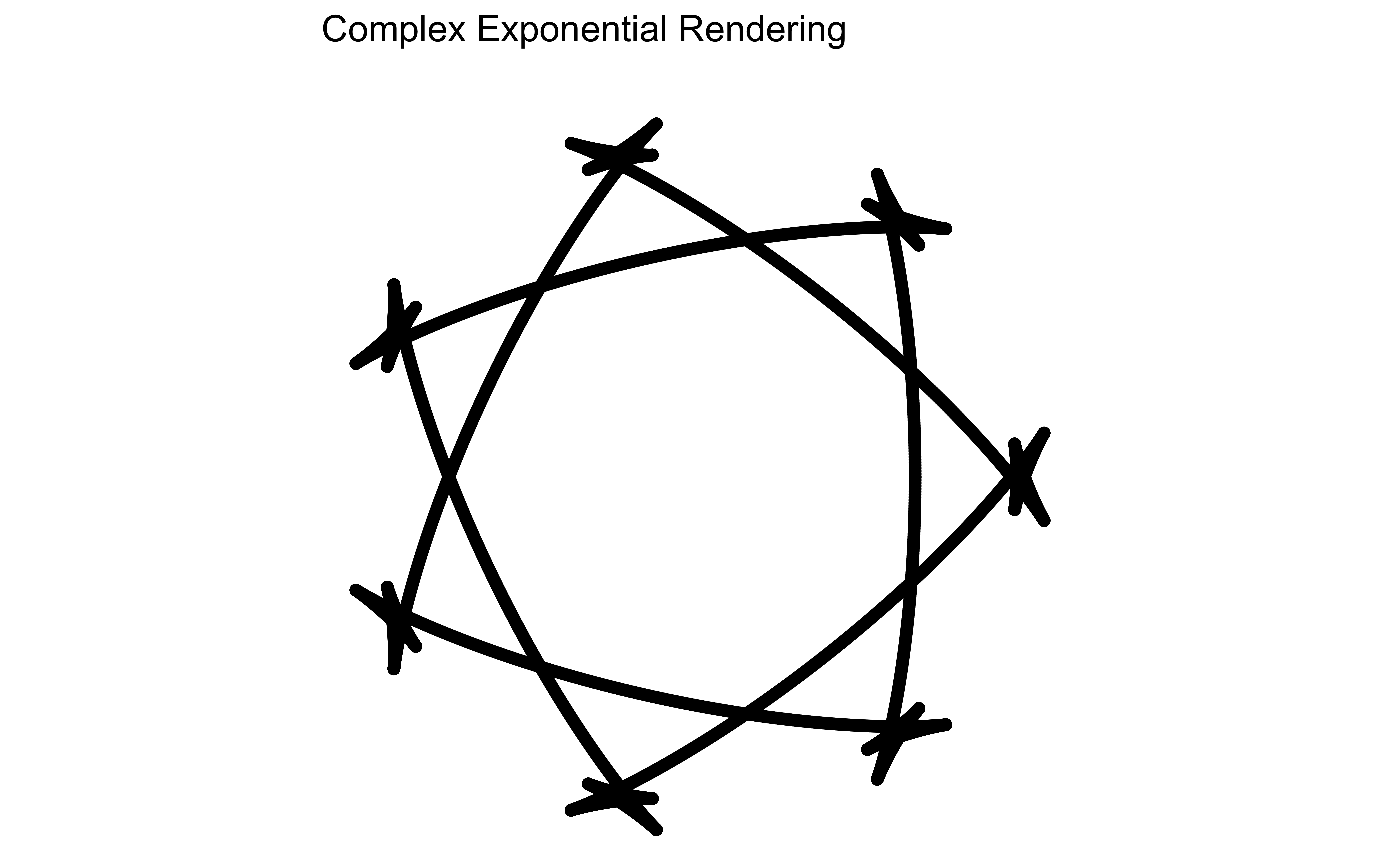
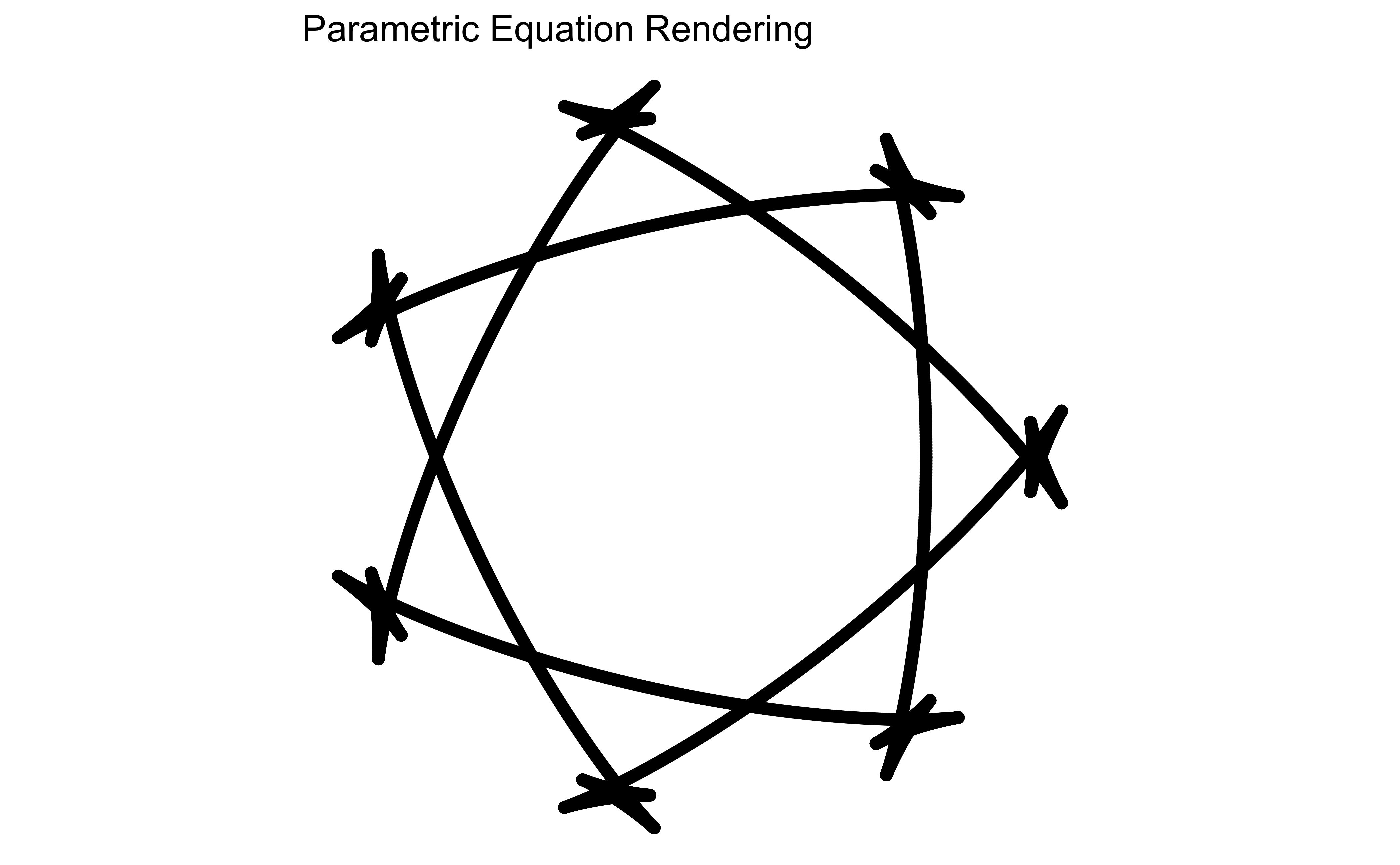
There, we have designed a pattern with seven-fold rotational symmetry. Can you make this in p5.js? Can you try for other orders and types of symmetry?
The coordinate system defines a positive increase in angle as the counterclockwise direction. So an increase in the parameter
Consider a small modification to our original Figure 1:
Show the Code
## Original Mystery Curve
# ## remainder = +1 from 5
# ## frequencies 1, 5+1, -15+1
data1 <- tibble::tibble(
  t = seq(0, 2 * pi, 0.001),
  x = cos(t) + cos(6 * t) / 2 + sin(14 * t) / 3,
  y = sin(t) + sin(6 * t) / 2 + cos(14 * t) / 3
)

# Mystery Curve
data1 %>%
  gf_point(y ~ x) %>%
  gf_refine(coord_equal()) %>%
  gf_theme(theme_void())
# Derived from Mystery
# Remainder = 2 from 5
# Frequencies: 2, 5+2, -15+2
# Coeffs: 1,1,1
data3 <- tibble::tibble(
  t = seq(0, 2 * pi, 0.001),
  x = cos(t) + cos(6 * t) + cos(14 * t),
  y = sin(t) + sin(6 * t) + sin(14 * t)
)
data3 %>%
  gf_point(y ~ x) %>%
  gf_refine(coord_equal()) %>%
  gf_hline(yintercept = 0) %>%
  gf_theme(theme_void())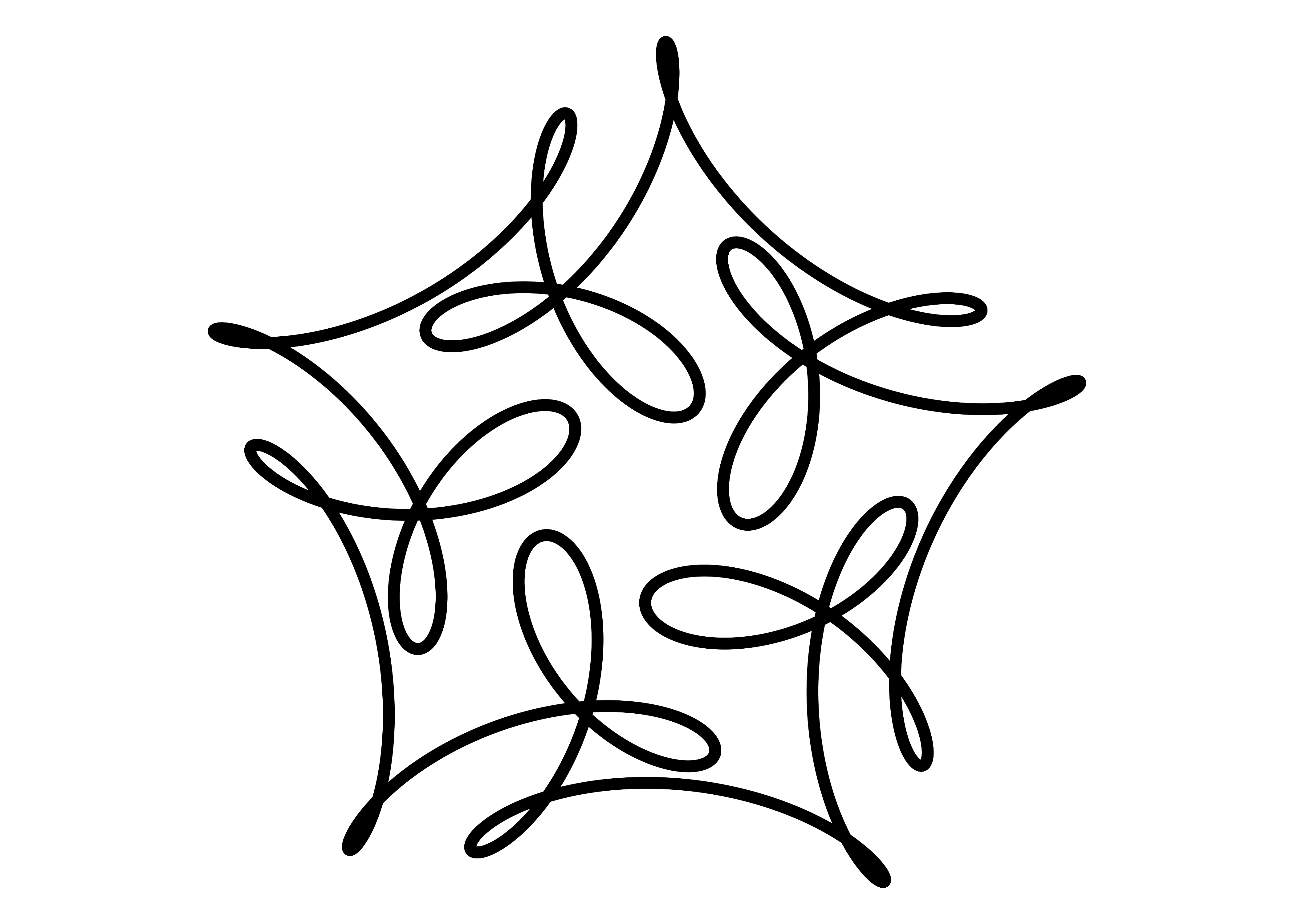
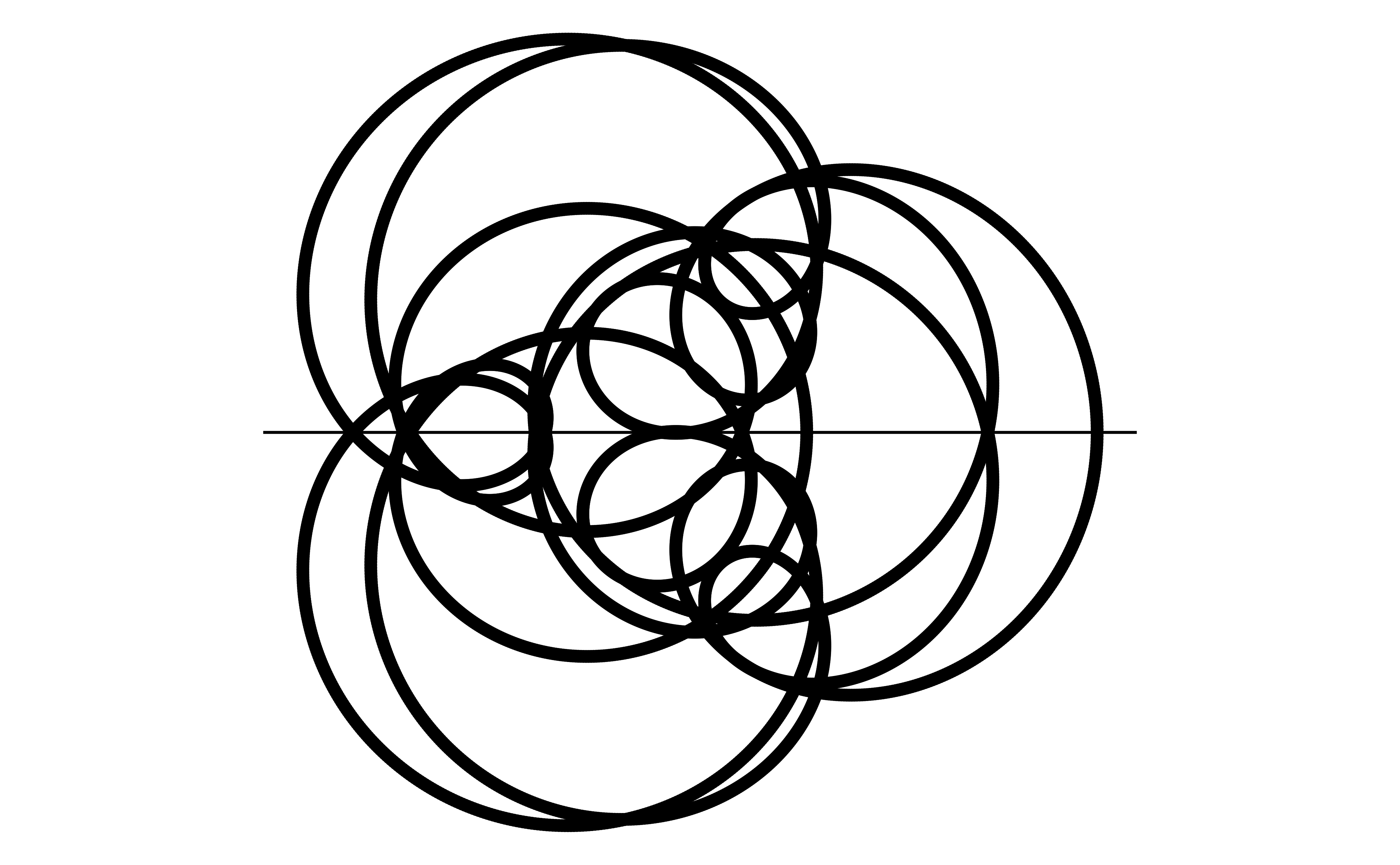
It should be immediately clear that the second pattern above is the same above and below the horizontal line; it exhibits horizontal mirror symmetry,
Under what conditions would a pattern be symmetric about an arbitrarily-tilted mirror, a mirror at angle
From Farris:
Mirror at Angle
When every coefficient is a real multiple of
The right-hand side is the correct expression for reflection across the line through the origin inclined at angle
Fun Extras to Try
It would be cool to simply develop the equations for any pattern in complex notation as in Equation 4 and throw that into code, without the tedious conversions into sines and cosines. Can we try that?
Here is an example in R:
Show the Code
t <- seq(0, 2 * pi, by = 0.001)
x <- t
## NOTE: need the minus sign here inside the exponential!!
## AND Absolutely need the "1" here before the solitary "i"!!
## Need to figure these out
f1 <- function(x) {
(exp(-(0 + 1i) * x) +
0.25 * exp(-(0 + 6i) * x) +
0.2 * exp(-(0 + 11i) * x))
}
plot(f1(x), asp = 1)
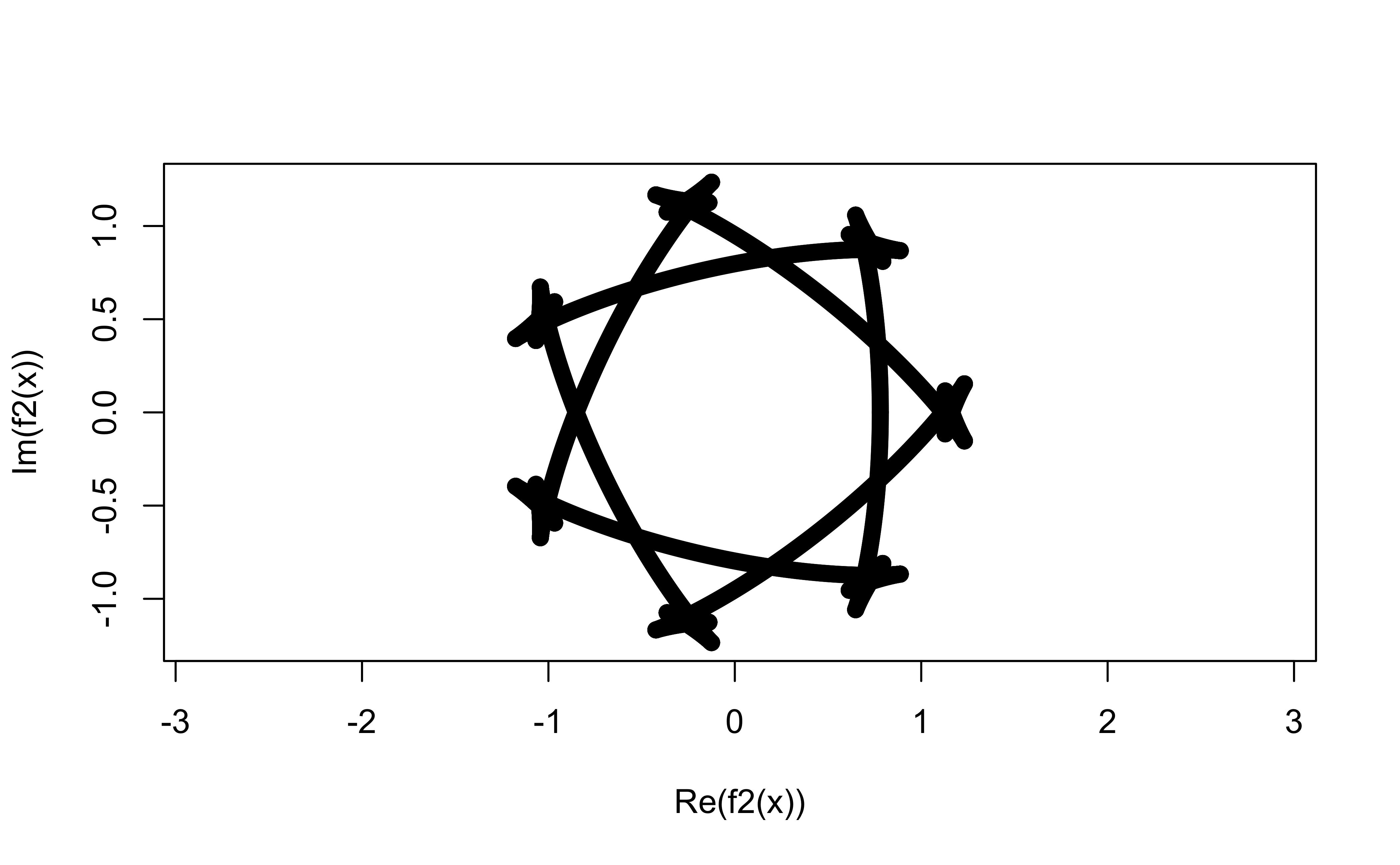
##
f2 <- function(x) {
(exp(-(0 + 2i) * x) +
0.2222 * exp(-(0 + 9i) * x) +
0.125 * exp(-(0 + 16i) * x) -
0.4 * exp(-(0 - 5i) * x) -
0.1667 * exp(-(0 - 12i) * x))
}
plot(f2(x), asp = 1)
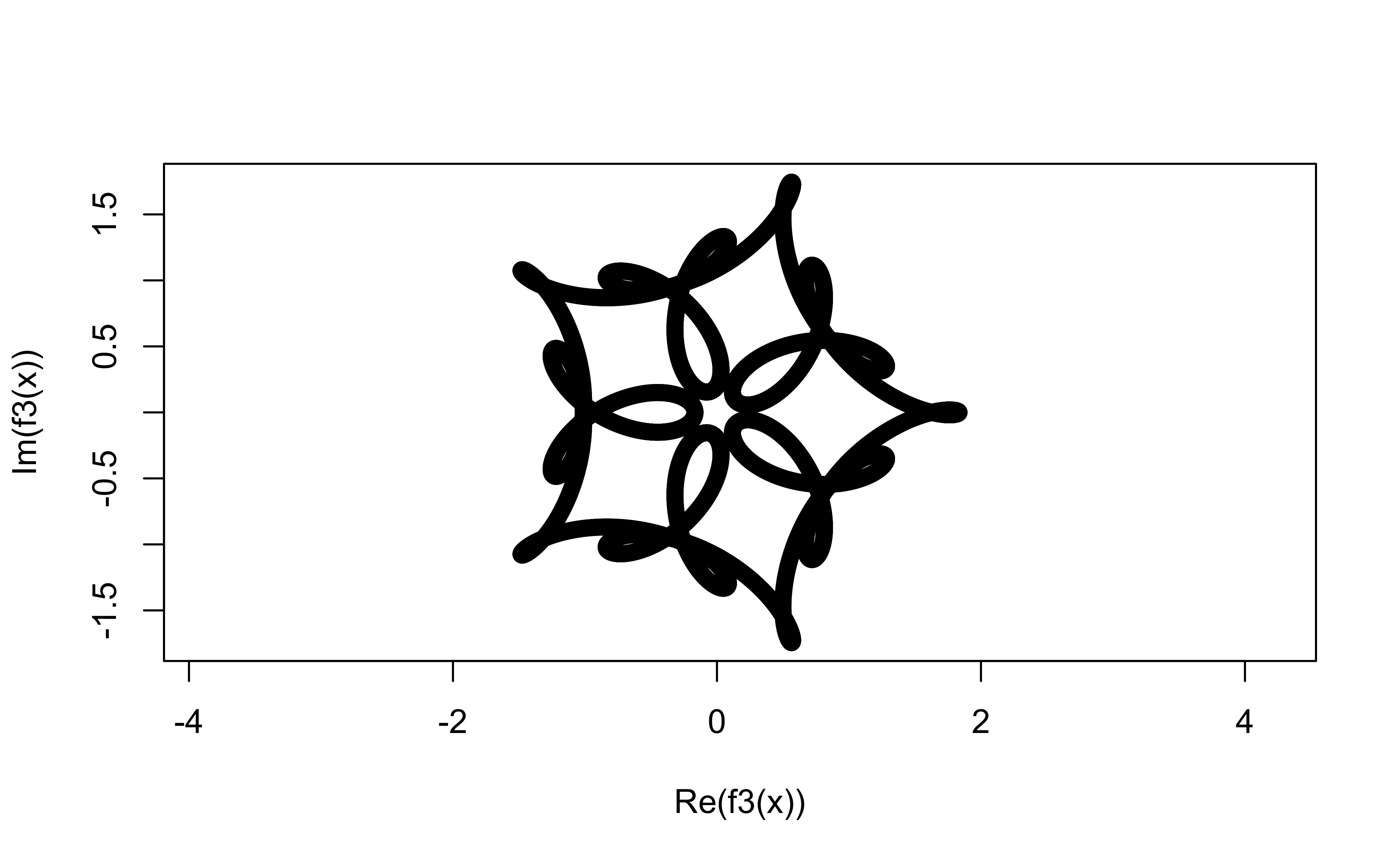
## Plotting with Exponential Functions
f3 <- function(x) {
(exp(-(0 + 1i) * x) +
0.5 * exp(-(0 + 6i) * x) +
1 / 3 * exp(-(0 - 14i) * x)
)
}
plot(f3(x), asp = 1)
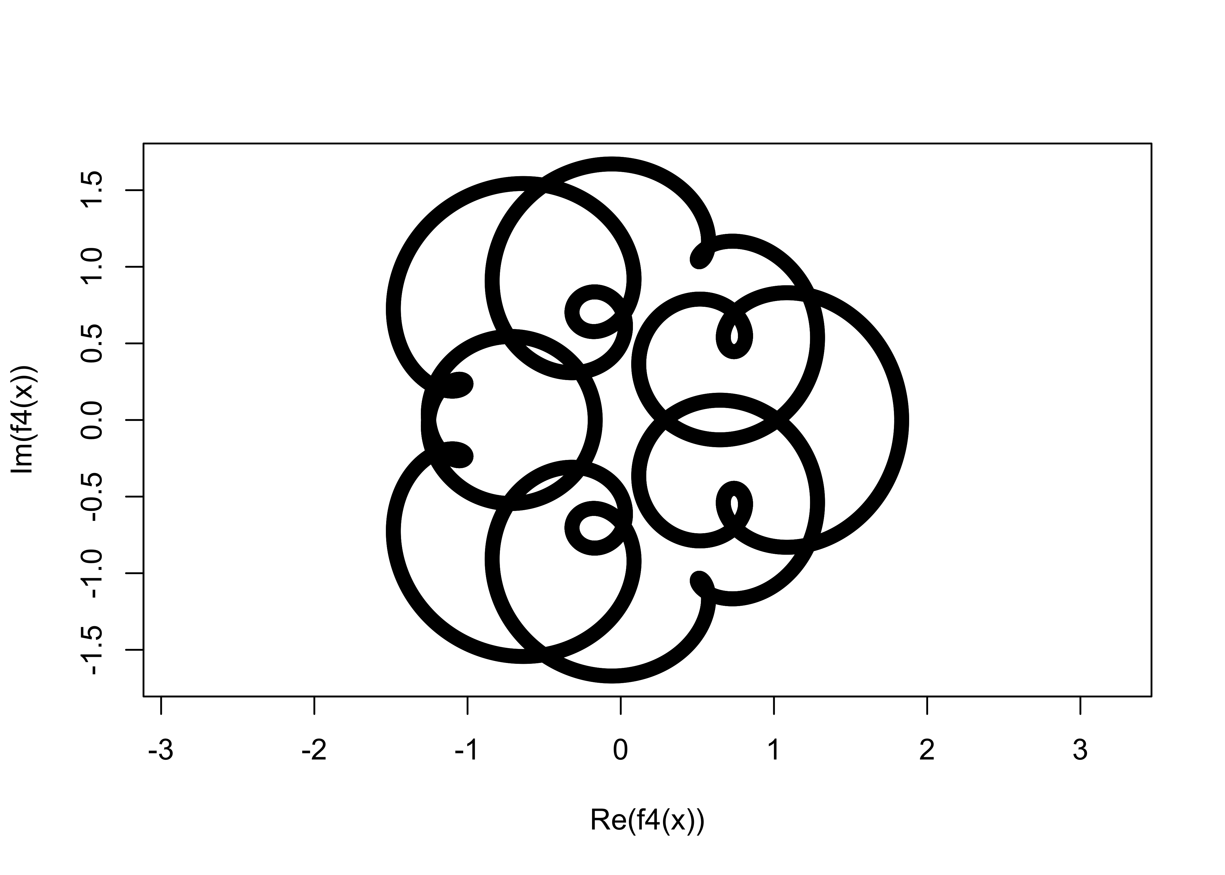
##
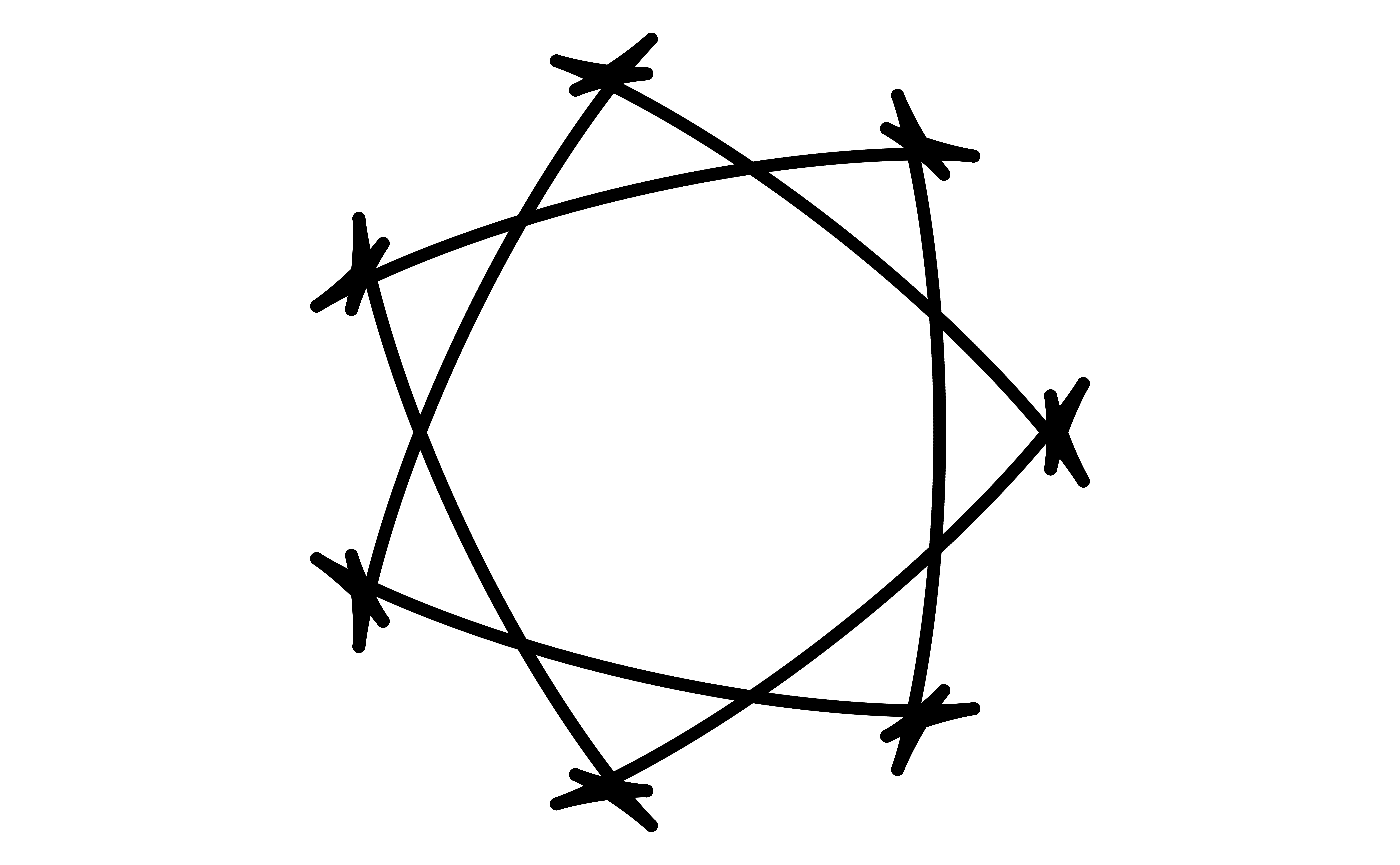
f4 <- function(x) {
(exp(-(0 + 1i) * x) +
0.5 * exp(-(0 + 6i) * x) +
1 / 3 * exp(-(0 + 14i) * x)
)
}
plot(f4(x), asp = 1)
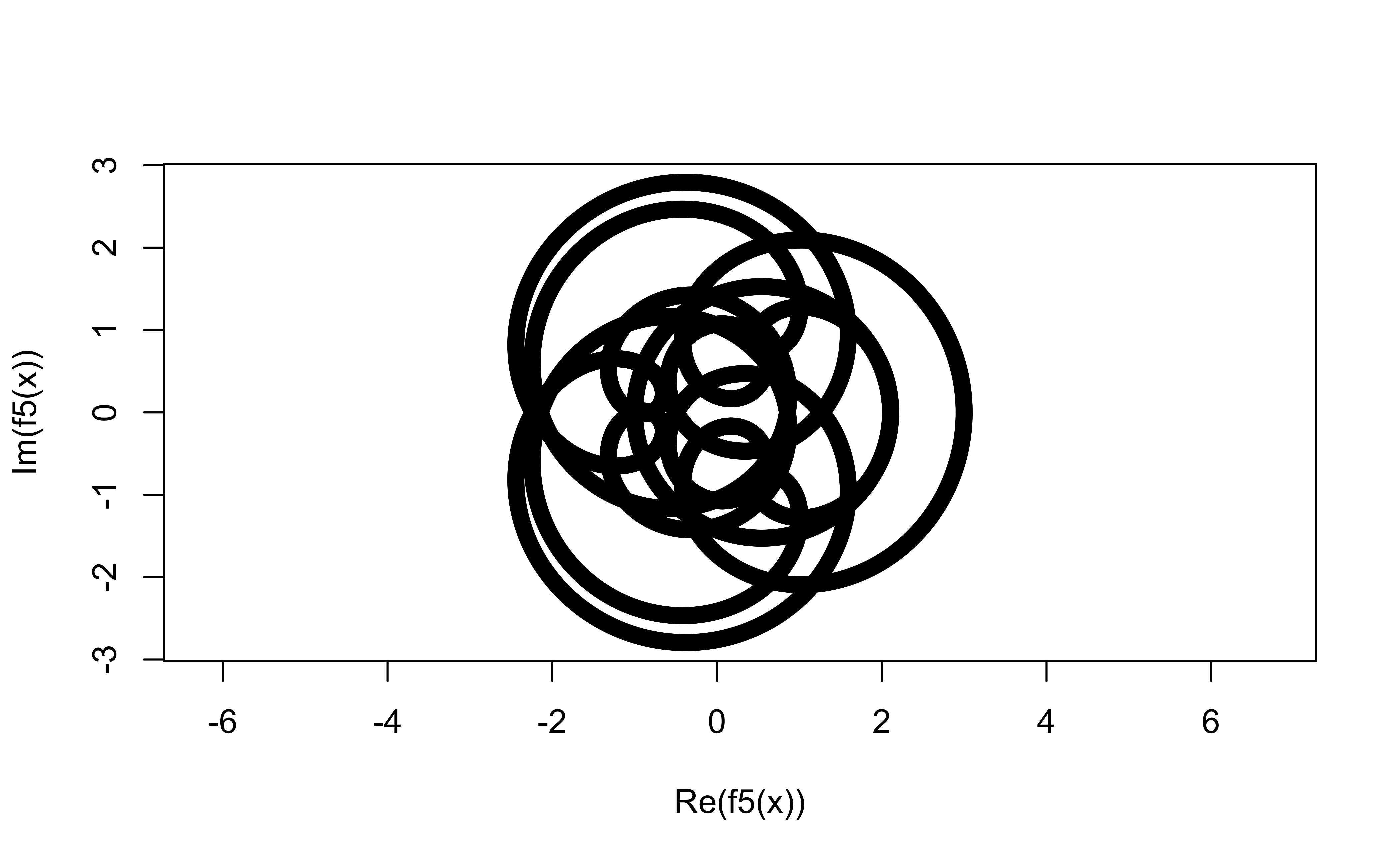
##
# ## remainder = +2 from 5
# ## frequencies 0+2, 5+2, -15+2
# ## Coefficients 1, 1, 1
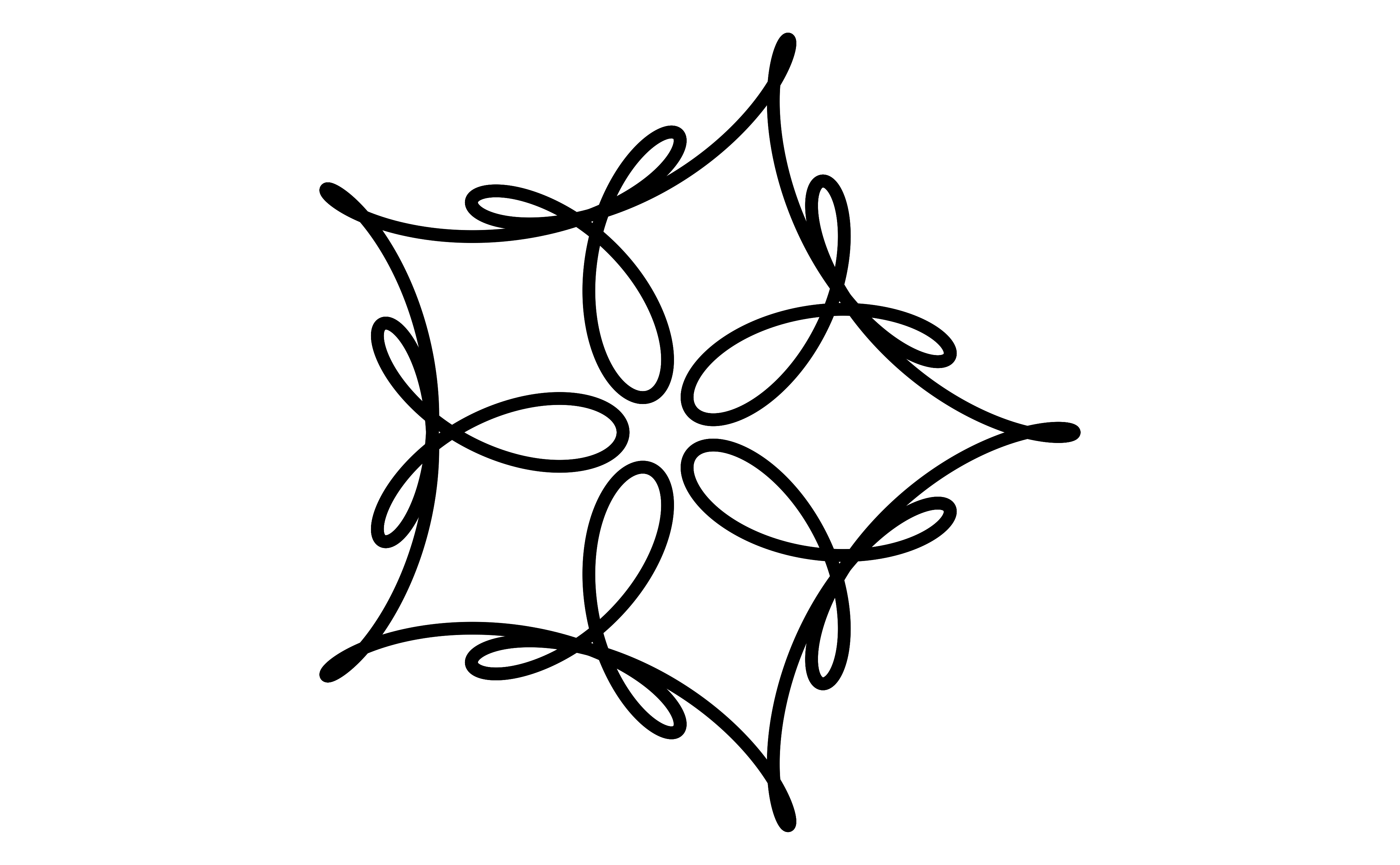
f5 <- function(x) {
(exp(-(0 + 2i) * x) +
1.0 * exp(-(0 + 7i) * x) +
1.0 * exp(-(0 + 13i) * x)
)
}
plot(f5(x), asp = 1)
##
# ## remainder = +2 from 5
# ## frequencies 0+2, 5+2, -15+2
# ## Coefficients 1, -1/2, -i/3 ( Note!!!)
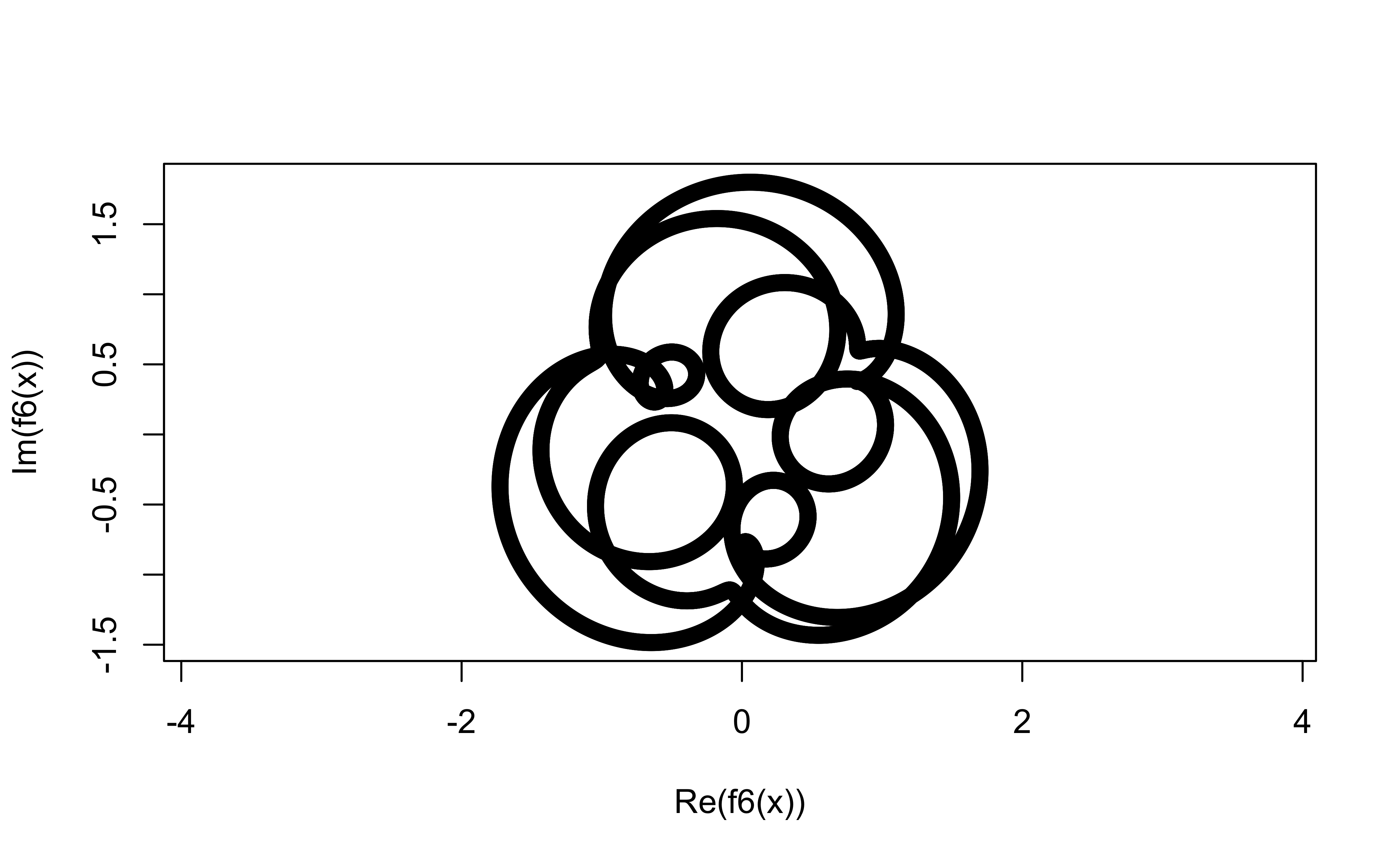
f6 <- function(x) {
(exp(-(0 + 2i) * x) +
-0.5 * exp(-(0 + 7i) * x) +
-1 / 3 * exp(pi / 2 * 1i) * exp(-(0 + 13i) * x)
)
}
plot(f6(x), asp = 1)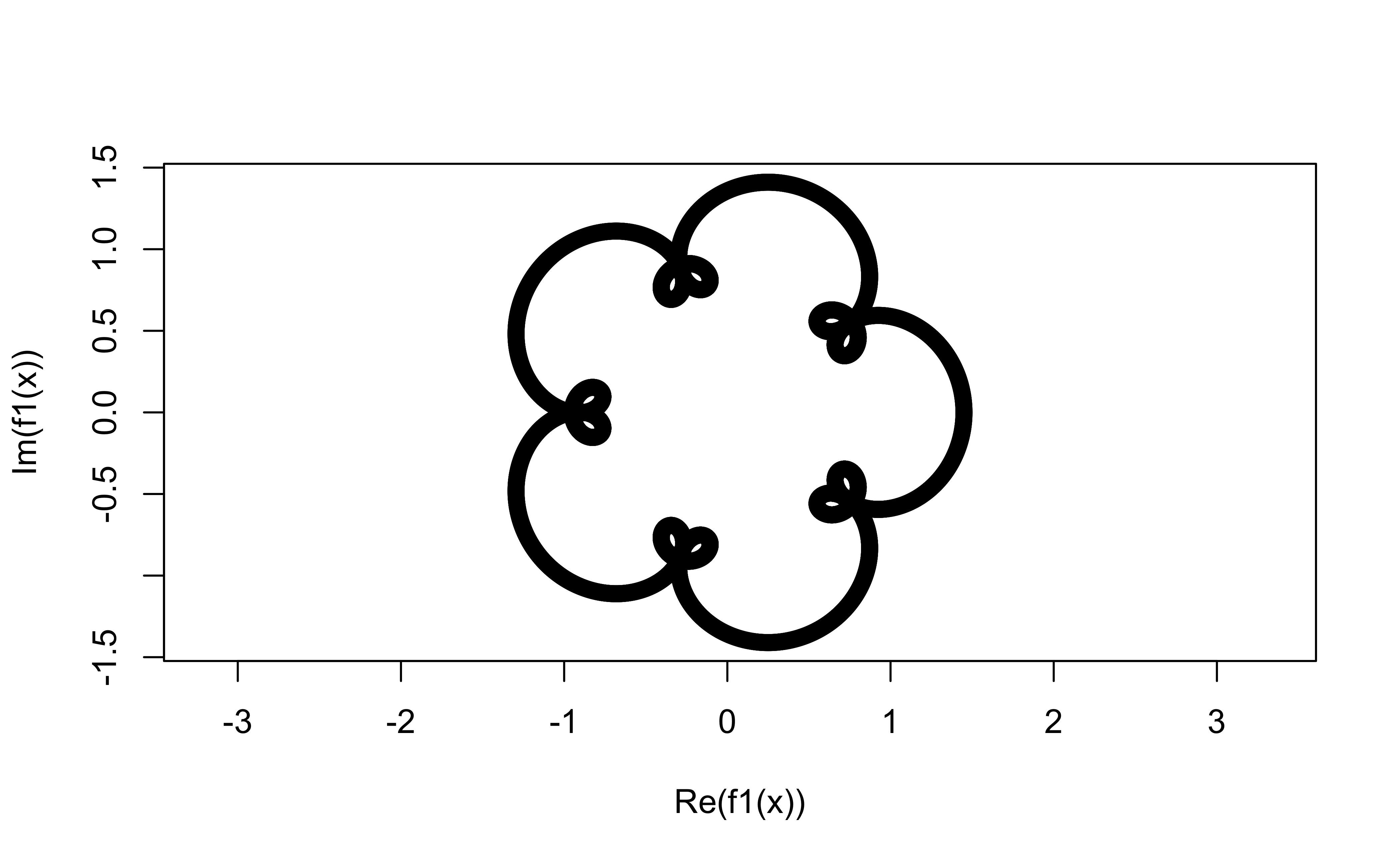
Show the Code
# t <- seq(0, 2 * pi, by = 0.001) # Already computed
data1 <- tibble(t, pattern = f1(t))
data2 <- tibble(t, pattern = f2(t))
data3 <- tibble(t, pattern = f3(t))
data4 <- tibble(t, pattern = f4(t))
data5 <- tibble(t, pattern = f5(t))
data6 <- tibble(t, pattern = f6(t))

data1 %>%
  gf_point(Im(pattern) ~ Re(pattern)) %>%
  gf_refine(coord_equal()) %>%
  gf_theme(theme_void())
data2 %>%
  gf_point(Im(pattern) ~ Re(pattern)) %>%
  gf_refine(coord_equal()) %>%
  gf_theme(theme_void())
data3 %>%
  gf_point(Im(pattern) ~ Re(pattern)) %>%
  gf_refine(coord_equal()) %>%
  gf_theme(theme_void())
data4 %>%
  gf_point(Im(pattern) ~ Re(pattern)) %>%
  gf_refine(coord_equal()) %>%
  gf_theme(theme_void())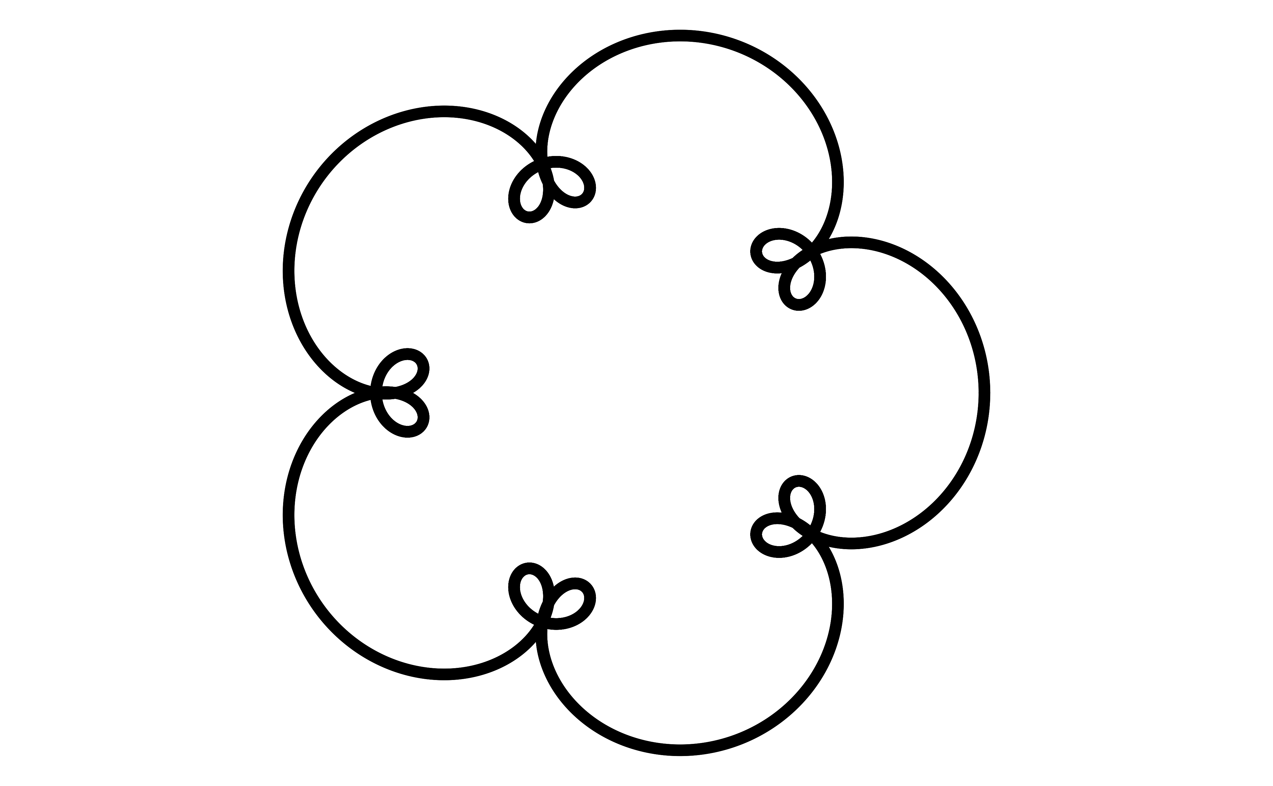
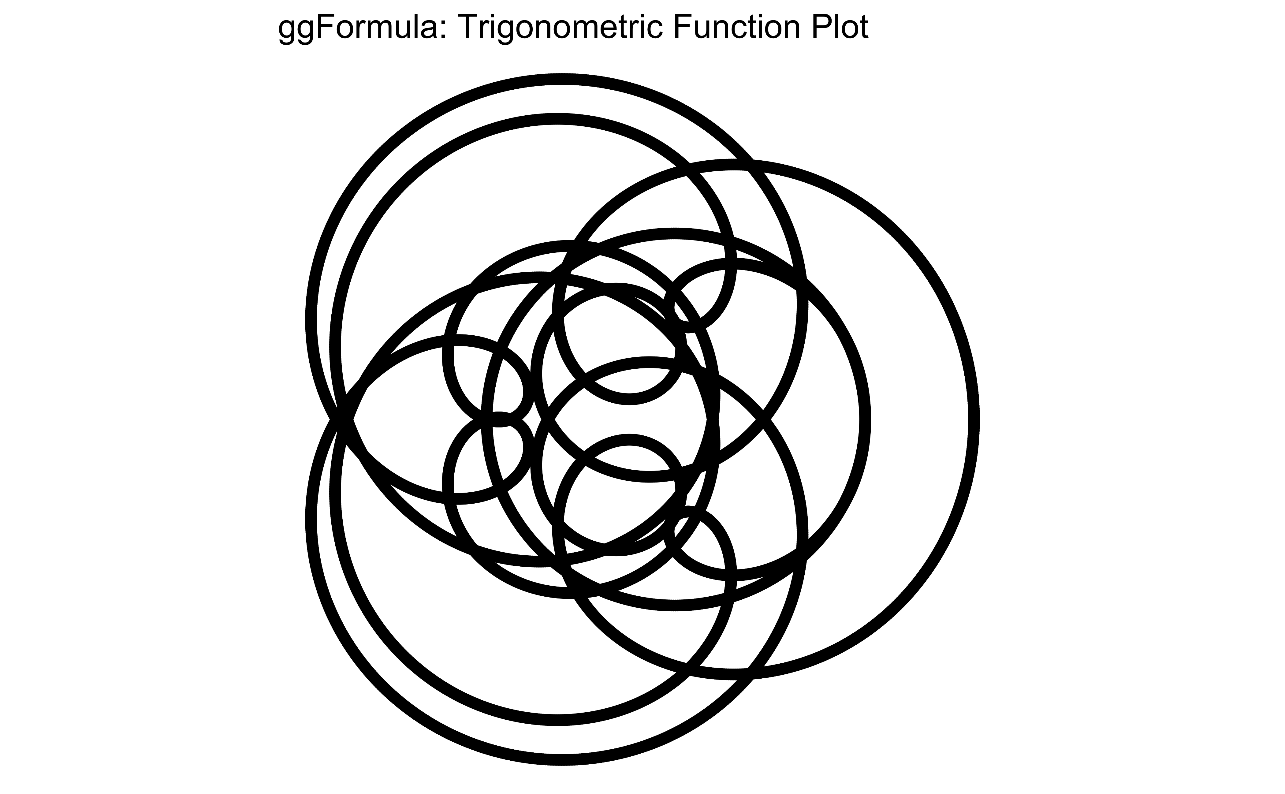
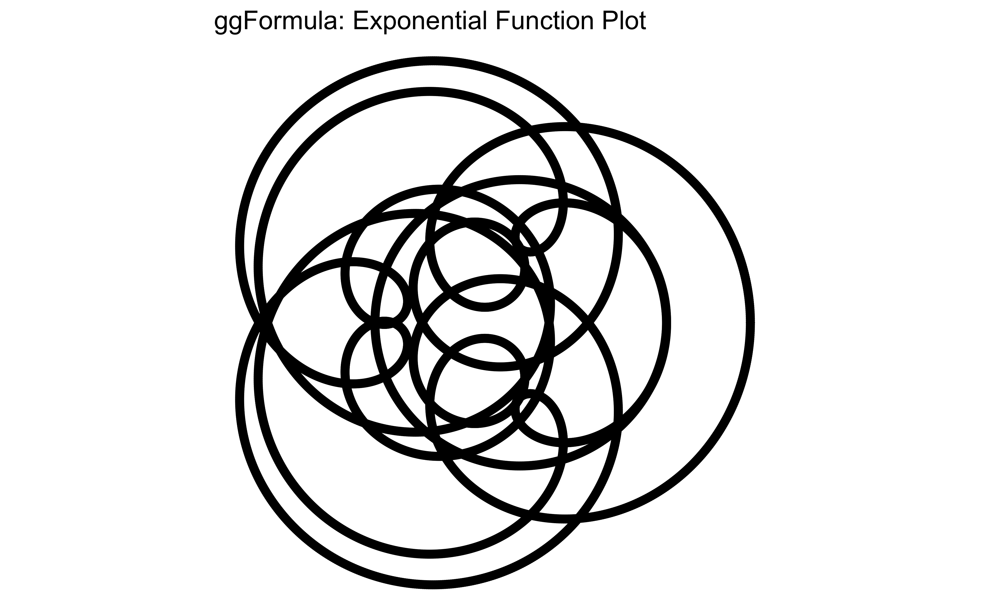
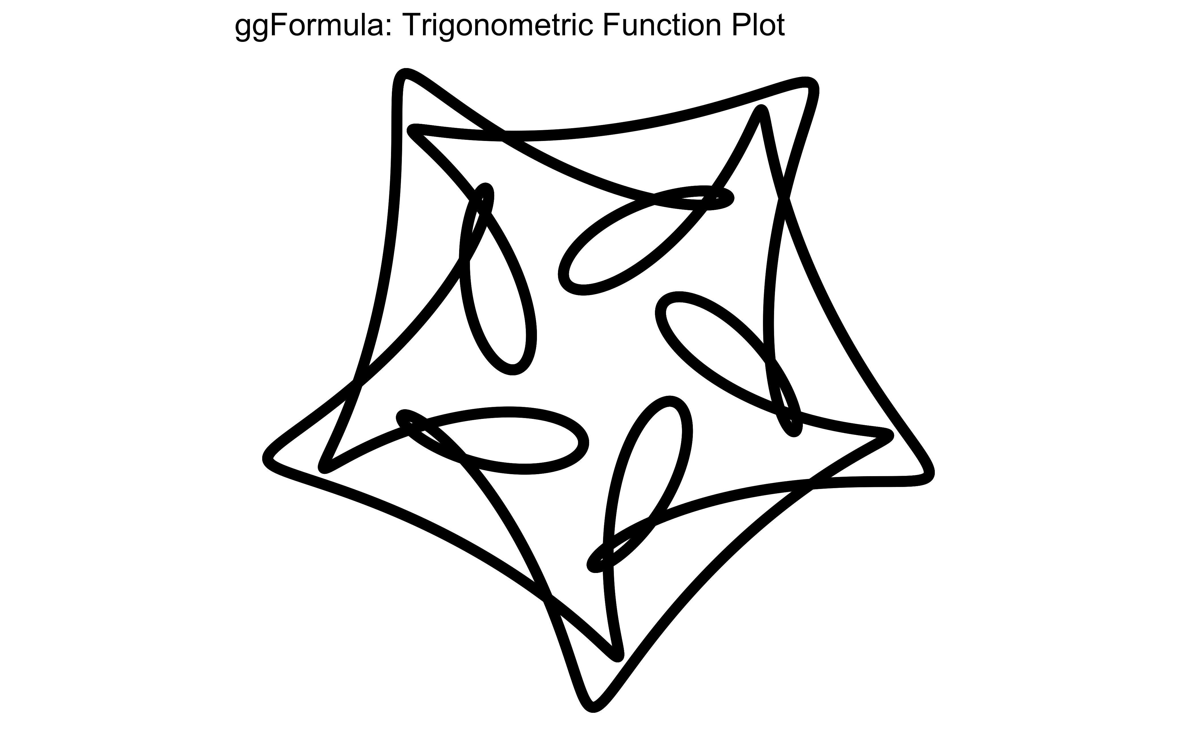
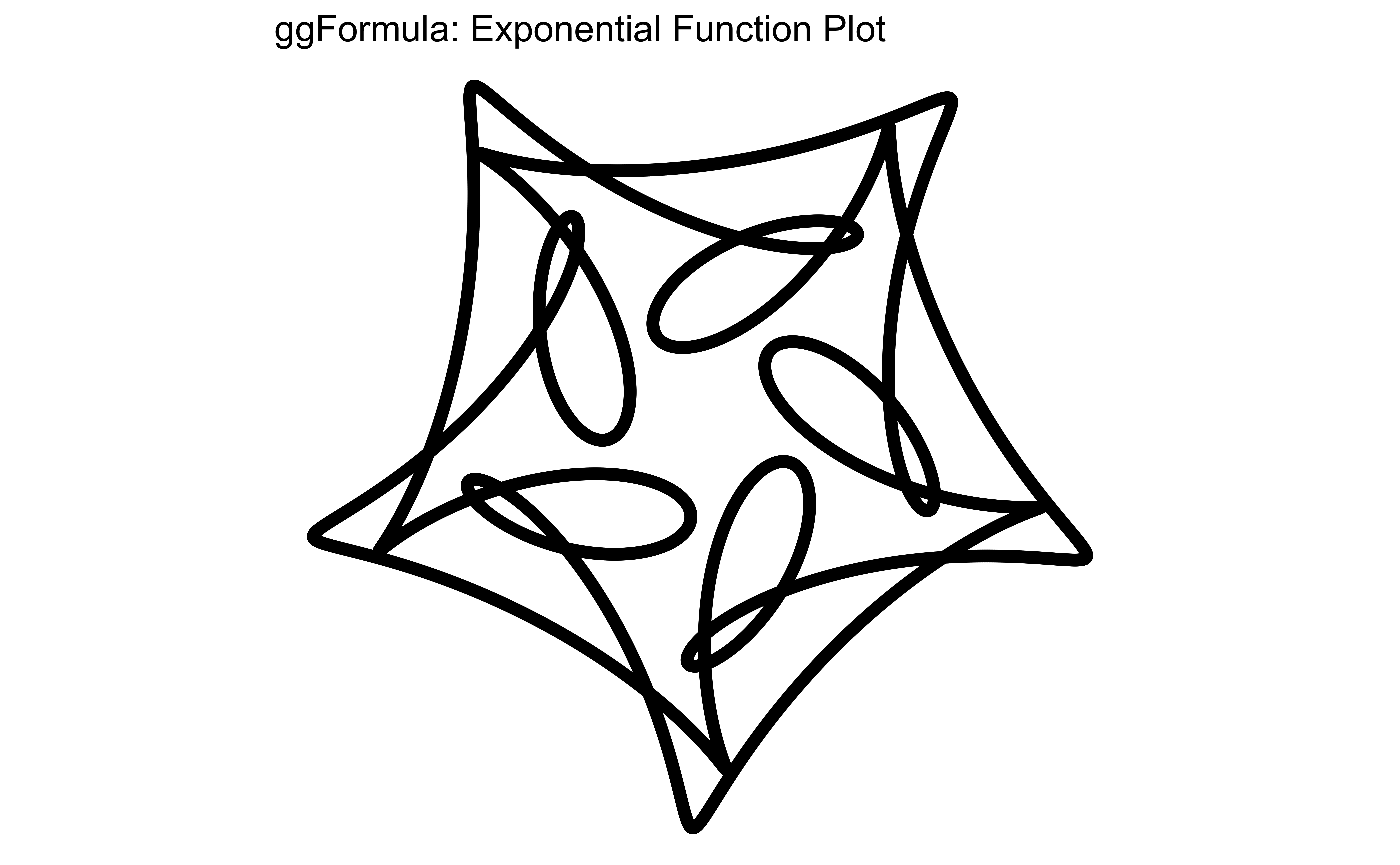
Comparing Exponential and Trigonometric Functions
Just for practice, let us once more be clear between the complex exponential notation, and the parametric trigonometric functions.
Show the Code
# ## remainder = +2 from 5
# ## frequencies 0+2, 5+2, -15+2
# ## Coefficients 1, 1, 1
f7 <- function(x) {
  (exp(-(0 + 2i) * x) + exp(-(0 + 7i) * x) + exp(-(0 + 13i) * x))
}

### Parametric Coordinates Tibble
data7a <- tibble::tibble(
  t = seq(0, 2 * pi, 0.001),
  x = cos((2) * t) + cos(7 * t) + cos(13 * t),
  y = sin(2 * t) + sin(7 * t) + sin(13 * t)
)
### Complex Exponential Tibble
data7b <- tibble(t, pattern = f7(t))
### Plots
plot(f7(x),
  asp = 1, cex = 0.2,
  main = "Base R: Exponential Function Plot"
)
###
data7a %>%
  gf_point(y ~ x,
    title = "ggFormula: Trigonometric Function Plot"
  ) %>%
  gf_refine(coord_equal()) %>%
  gf_theme(theme_void())
###
data7b %>%
  gf_point(Im(pattern) ~ Re(pattern),
    title = "ggFormula: Exponential Function Plot"
  ) %>%
  gf_refine(coord_equal()) %>%
  gf_theme(theme_void())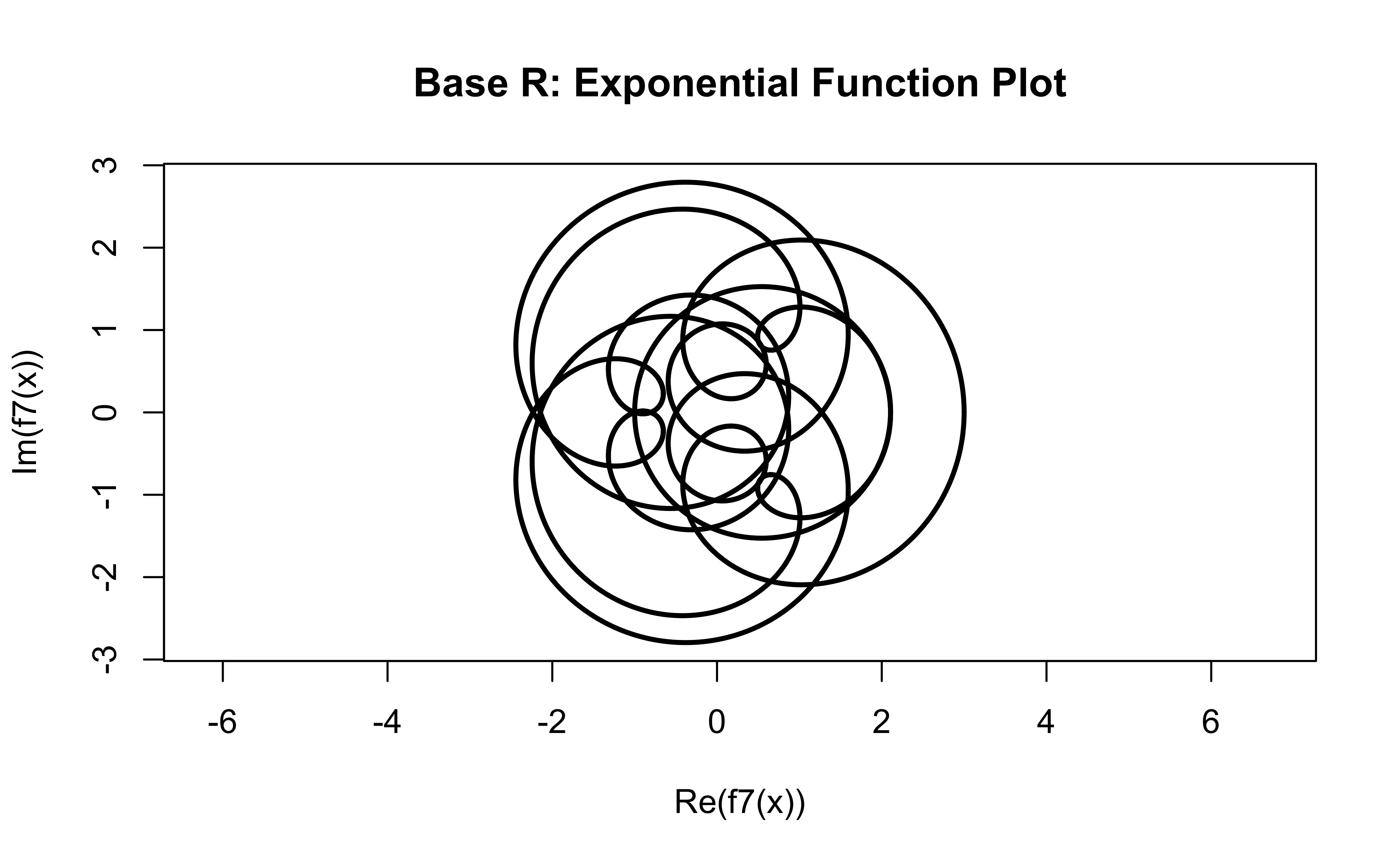
Show the Code
# ## remainder = +2 from 5
# ## frequencies 0+2, 5+2, -15+2
# ## Coefficients 1, -1/2, -i/3 ( Note!!!)
f8 <- function(x) {
  (exp(-(0 + 2i) * x) - 0.5 * exp(-(0 + 7i) * x) +
    1i / 3 * exp((0 + 13i) * x))
}

data8a <- tibble::tibble(
  t = seq(0, 2 * pi, 0.001),
  x = cos(2 * t) - 0.5 * cos(7 * t) +
    0.3 * cos(-13 * t + pi / 2),
  y = sin(2 * t) - 0.5 * sin(7 * t) +
    0.3 * sin(-13 * t + pi / 2)
)
data8b <- tibble(t, pattern = f8(t))
###
plot(f8(x),
  asp = 1, cex = 0.2,
  main = "Base R: Exponential Function Plot"
)
###
data8a %>%
  gf_point(y ~ x, title = "ggFormula: Trigonometric Function Plot") %>%
  gf_refine(coord_equal()) %>%
  gf_theme(theme_void())
###
data8b %>%
  gf_point(Im(pattern) ~ Re(pattern),
    title = "ggFormula: Exponential Function Plot"
  ) %>%
  gf_refine(coord_equal()) %>%
  gf_theme(theme_void())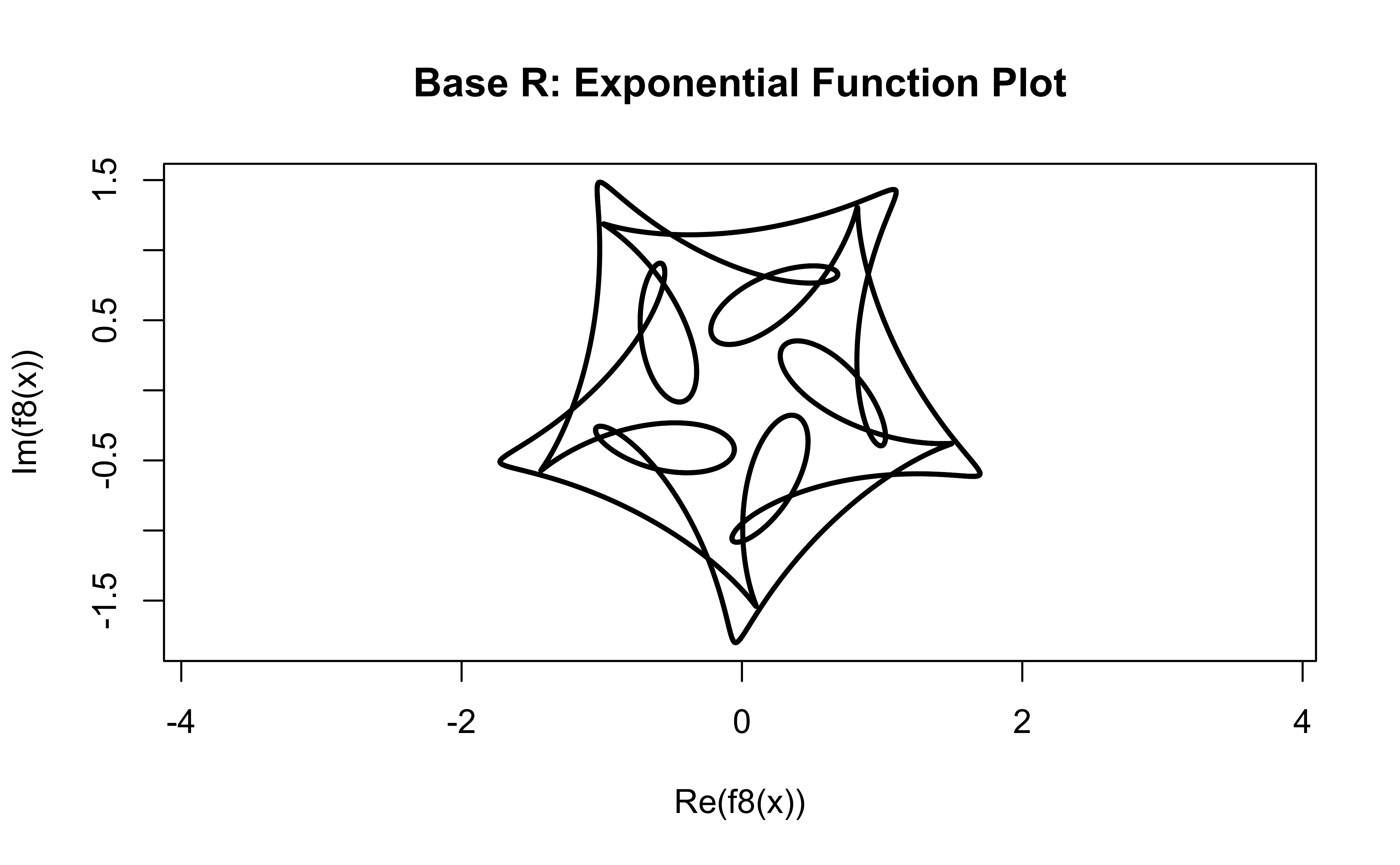
Sums of Complex exponentials are very common in mathematics and show up in many places: here, with symmetry, with Fourier Series, with Sound synthesis and Analysis.
We have seen the close relationship between complex rotating exponentials and their trigonometric decompositions, embodied in the Euler Formula.
We also saw how multiple such exponentials can be used to combine using complex weighting to create symmetric patterns.
And how symmetry depends upon the frequencies of the exponentials having a very specific relationship using modulo arithmetic.
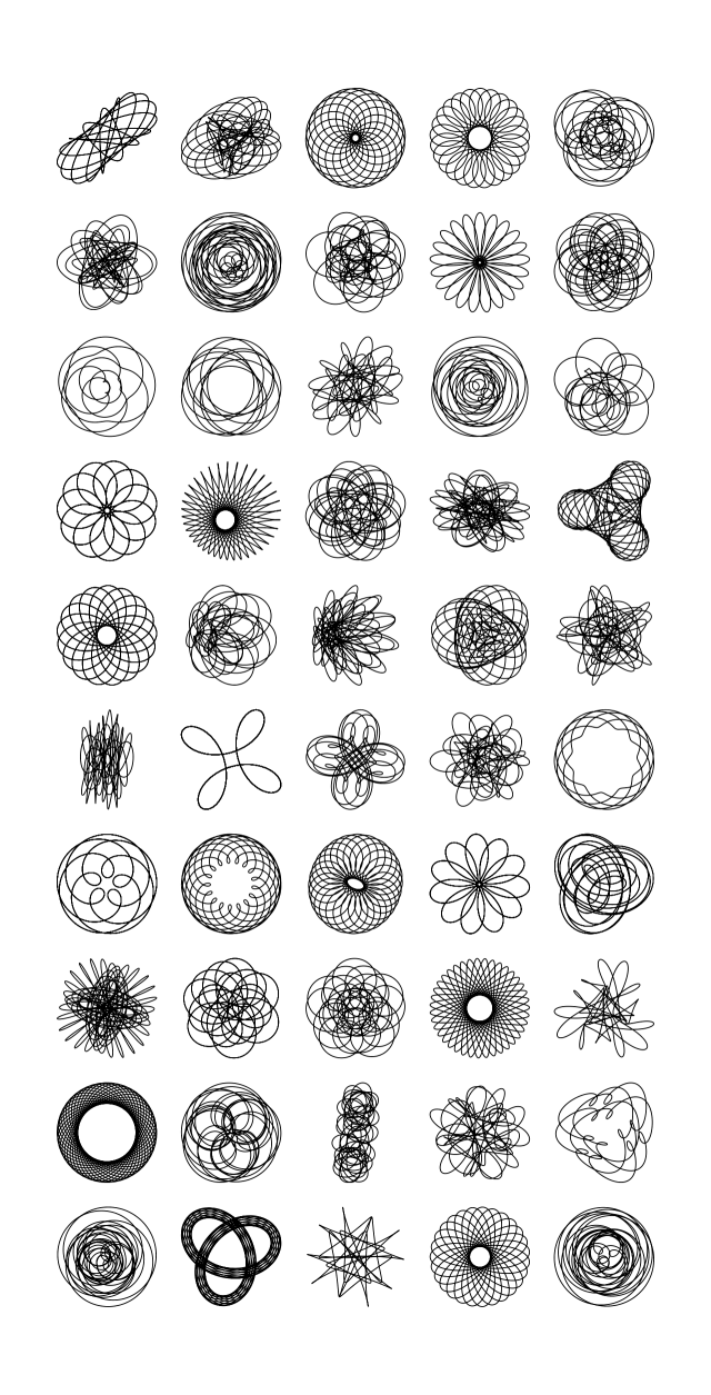
Your Turn
Can you reverse engineer these curves, in R or in p5.js?
- Frank Farris. Creating Symmetry: The Artful Mathematics of Wallpaper Patterns. Princeton University Press (2 June 2015).
- Doga Kurkcuoglu. https://bilimneguzellan.net/en/follow-up-to-fourier-series-2/. Look at some very cool animations here!
- Gorilla Sun Blog. https://www.gorillasun.de/blog/parametric-functions-and-particles/
- CrateCode: Complex Generative Art with p5.js. https://cratecode.com/info/p5js-generative-art-complex-functions
- Gorilla Sun Blog. https://www.gorillasun.de/blog/parametric-functions-and-particles/
- Brent Yorgey.(2015). The Math Less Travelled Blog. Random Cylic Curves. https://mathlesstraveled.wordpress.com/2015/06/04/random-cyclic-curves-5/
- University of New South wales. Exponential Sums Page. https://www.unsw.edu.au/science/our-schools/maths/our-school/spotlight-on-our-people/history-school/glimpses-mathematics-and-statistics/exponential-sums
- John Myles White. Complex Numbers in R. https://www.johnmyleswhite.com/notebook/2009/12/18/using-complex-numbers-in-r/
| Package | Version | Citation |
|---|---|---|
| ggformula | 0.12.0 | Kaplan and Pruim (2023) |
Kaplan, Daniel, and Randall Pruim. 2023. ggformula: Formula Interface to the Grammar of Graphics. https://doi.org/10.32614/CRAN.package.ggformula.
Citation
BibTeX citation:
@online{2024,
  author = {},
  title = {\textless Iconify-Icon Icon=“ph:circles-Three-Fill”
    Width=“1.2em”
    Height=“1.2em”\textgreater\textless/Iconify-Icon\textgreater{}
    \textless Iconify-Icon Icon=“gravity-Ui:function” Width=“1.2em”
    Height=“1.2em”\textgreater\textless/Iconify-Icon\textgreater{}
    {Circles}},
  date = {2024-05-02},
  url = {https://av-quarto.netlify.app/content/courses/MathModelsDesign/Modules/25-Geometry/10-Circles/},
  langid = {en}
}
For attribution, please cite this work as:
“<Iconify-Icon Icon=‘ph:circles-Three-Fill’
Width=‘1.2em’
Height=‘1.2em’></Iconify-Icon> <Iconify-Icon
Icon=‘gravity-Ui:function’ Width=‘1.2em’
Height=‘1.2em’></Iconify-Icon> Circles.”
2024. May 2, 2024. https://av-quarto.netlify.app/content/courses/MathModelsDesign/Modules/25-Geometry/10-Circles/.