Lab-12: Time is a Him!!

Time Series in R

Line Charts

Boxplot Charts

Heatmaps

Averaging

Predictions

Exponential Smoothing

ARIMA models

Forecasting

Author

Arvind Venkatadri

Published

February 14, 2022

Modified

June 12, 2025

Introduction

Time Series data are important in data visualization where events have a temporal dimension, such as with finance, transportation, music, telecommunications for example.

library(tidyverse)
library(mosaic)
library(ggformula)
##########################################
# Install core TimeSeries Packages
# library(ctv)
# ctv::install.views("TimeSeries", coreOnly = TRUE)
# To update core TimeSeries packages
# ctv::update.views("TimeSeries")
# Time Series Core Packages
##########################################
library(tsibble)
library(feasts) # Feature Extraction and Statistics for Time Series
library(fable) # Forecasting Models for Tidy Time Series
library(tseries) # Time Series Analysis and Computational Finance
library(forecast)
library(zoo)
##########################################
library(tsibbledata) # Time Series Demo Datasets
## New package from Mitchell Ohara-Wild in June 2025
library(ggtime)

Introduction to Time Series: Data Formats

There are multiple formats for time series data.

The base ts format: The stats::ts() function will convert a numeric vector into an R time series object. The format is ts(vector, start=, end=, frequency=) where start and end are the times of the first and last observation and frequency is the number of observations per unit time (1=annual, 4=quarterly, 12=monthly, etc.). Used by established packages like forecast
Tibble format: the simplest is of course the standard tibble / dataframe, with a time variable to indicate that the other variables vary with time. Used by more recent packages such as timetk & modeltime
The modern tsibble (time series tibble) format: this is a new format for time series analysis, and is used by the tidyverts set of packages (fable, feasts and others).
There is also a tsbox package from ROpenScience that allows easy inter-conversion between these ( and other! ) formats!

Creating time series

In this first example, we will use simple ts data, and then do another with a tibble dataset, and then a third example with an tsibble formatted dataset.

`ts` format data

There are a few datasets in base R that are in ts format already.

AirPassengers

     Jan Feb Mar Apr May Jun Jul Aug Sep Oct Nov Dec
1949 112 118 132 129 121 135 148 148 136 119 104 118
1950 115 126 141 135 125 149 170 170 158 133 114 140
1951 145 150 178 163 172 178 199 199 184 162 146 166
1952 171 180 193 181 183 218 230 242 209 191 172 194
1953 196 196 236 235 229 243 264 272 237 211 180 201
1954 204 188 235 227 234 264 302 293 259 229 203 229
1955 242 233 267 269 270 315 364 347 312 274 237 278
1956 284 277 317 313 318 374 413 405 355 306 271 306
1957 315 301 356 348 355 422 465 467 404 347 305 336
1958 340 318 362 348 363 435 491 505 404 359 310 337
1959 360 342 406 396 420 472 548 559 463 407 362 405
1960 417 391 419 461 472 535 622 606 508 461 390 432

str(AirPassengers)

 Time-Series [1:144] from 1949 to 1961: 112 118 132 129 121 135 148 148 136 119 ...

This can be easily plotted using base R:

plot(AirPassengers)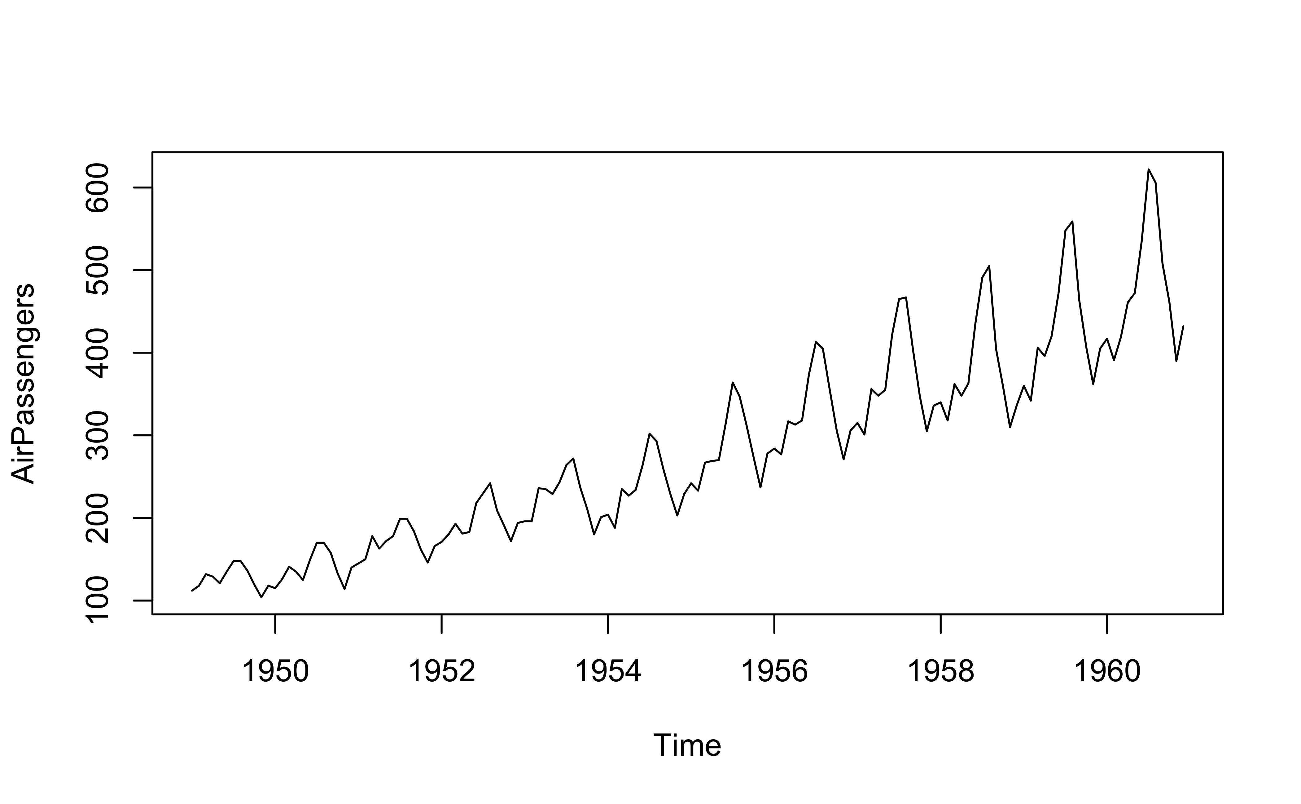

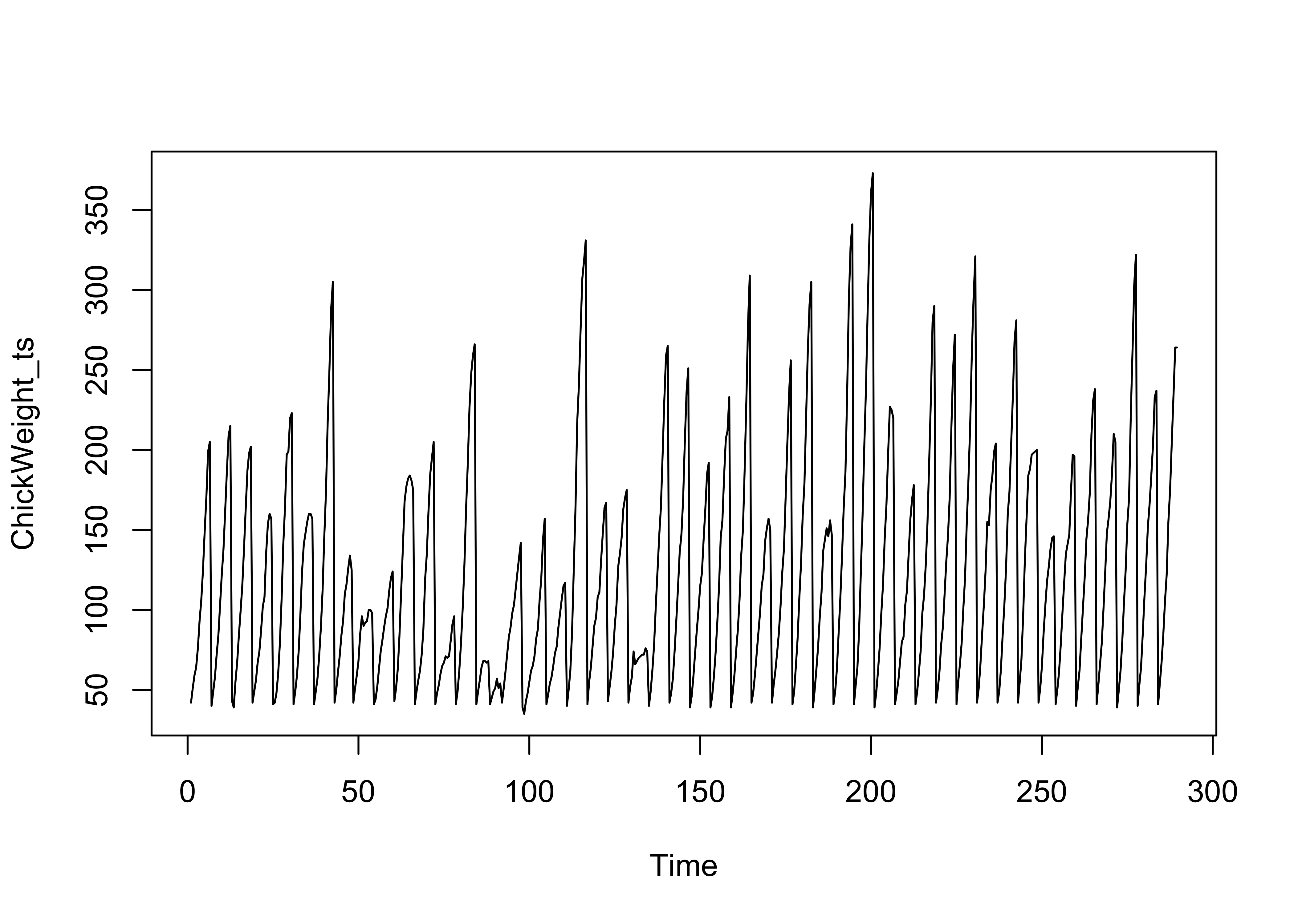
Let us take data that is “time oriented” but not in ts format, and convert it to ts: the syntax of ts() is:

Syntax: objectName <- ts(data, start, end, frequency) where - data represents the data vector - start represents the first observation in time series
- end represents the last observation in time series
- frequency represents number of observations per unit time. For example, frequency=1 for monthly data.

We will pick simple numerical vector data ( i.e. not a timeseries ) ChickWeight:

ChickWeight %>% head()

ABCDEFGHIJ0123456789

	weight <dbl>	Time <dbl>	Chick <ord>	Diet <fct>
1	42	0	1	1
2	51	2	1	1
3	59	4	1	1
4	64	6	1	1
5	76	8	1	1
6	93	10	1	1

ChickWeight_ts <- ts(ChickWeight$weight, frequency = 2)
plot(ChickWeight_ts)

The ts format

The ts format is not recommended for new analysis since it does not permit inclusion of multiple time series in one dataset, nor other categorical variables for grouping etc.

`tibble` format data

Some “time-oriented” datasets are available in tibble form. Let us try to plot one, the walmart_sales_weekly dataset from the timetk package:

data(walmart_sales_weekly, package = "timetk")
walmart_sales_weekly

ABCDEFGHIJ0123456789

id <fct>	Store <dbl>	Dept <dbl>	Date <date>	Weekly_Sales <dbl>	IsHoliday <lgl>	Type <chr>	Size <dbl>	Temperature <dbl>	Fuel_Price <dbl>
1_1	1	1	2010-02-05	24924.50	FALSE	A	151315	42.31	2.572
1_1	1	1	2010-02-12	46039.49	TRUE	A	151315	38.51	2.548
1_1	1	1	2010-02-19	41595.55	FALSE	A	151315	39.93	2.514
1_1	1	1	2010-02-26	19403.54	FALSE	A	151315	46.63	2.561
1_1	1	1	2010-03-05	21827.90	FALSE	A	151315	46.50	2.625
1_1	1	1	2010-03-12	21043.39	FALSE	A	151315	57.79	2.667
1_1	1	1	2010-03-19	22136.64	FALSE	A	151315	54.58	2.720
1_1	1	1	2010-03-26	26229.21	FALSE	A	151315	51.45	2.732
1_1	1	1	2010-04-02	57258.43	FALSE	A	151315	62.27	2.719
1_1	1	1	2010-04-09	42960.91	FALSE	A	151315	65.86	2.770

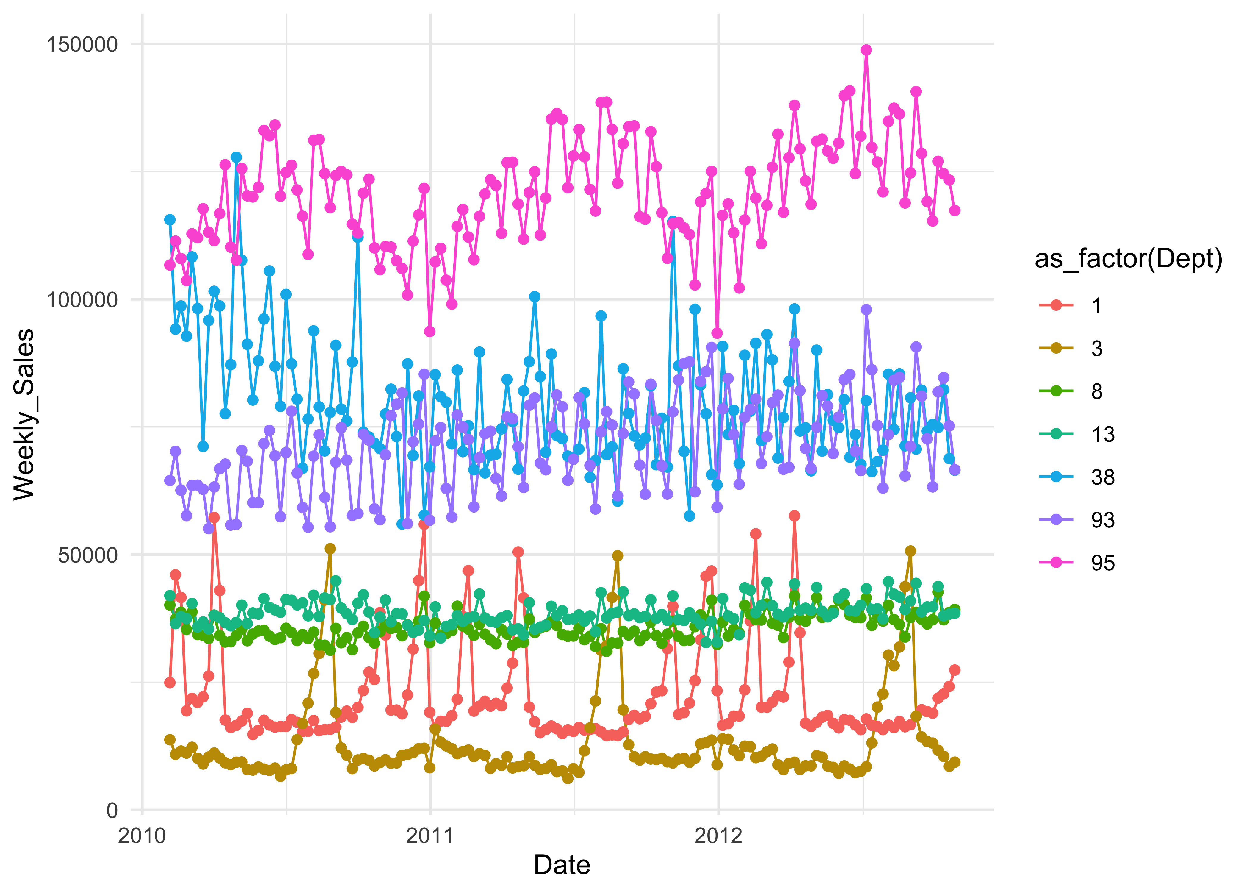
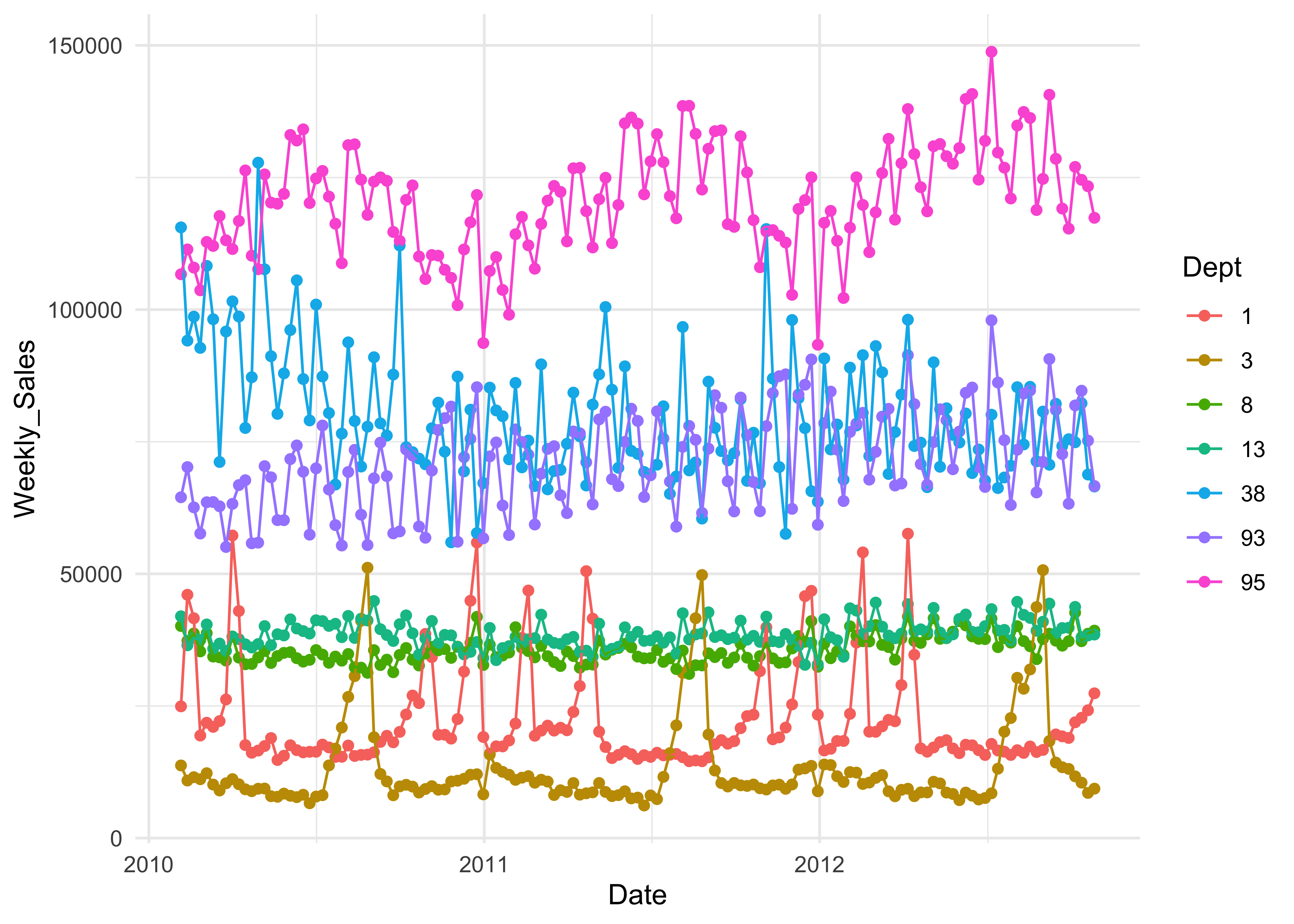
This dataset is a tibble with a Date column. The Dept column is clearly a categorical column that allows us to distinguish separate time series, i.e. one for each value of Dept. We will convert that to a factor( it is an double precision number ) and then plot the data using this column on the Date on the $x$ -axis:

walmart_sales_weekly %>%
  # convert Dept number to a **categorical factor**
  mutate(Dept = forcats::as_factor(Dept)) %>%
  gf_point(Weekly_Sales ~ Date,
    group = ~Dept,
    colour = ~Dept, data = .
  ) %>%
  gf_line() %>%
  gf_theme(theme_minimal())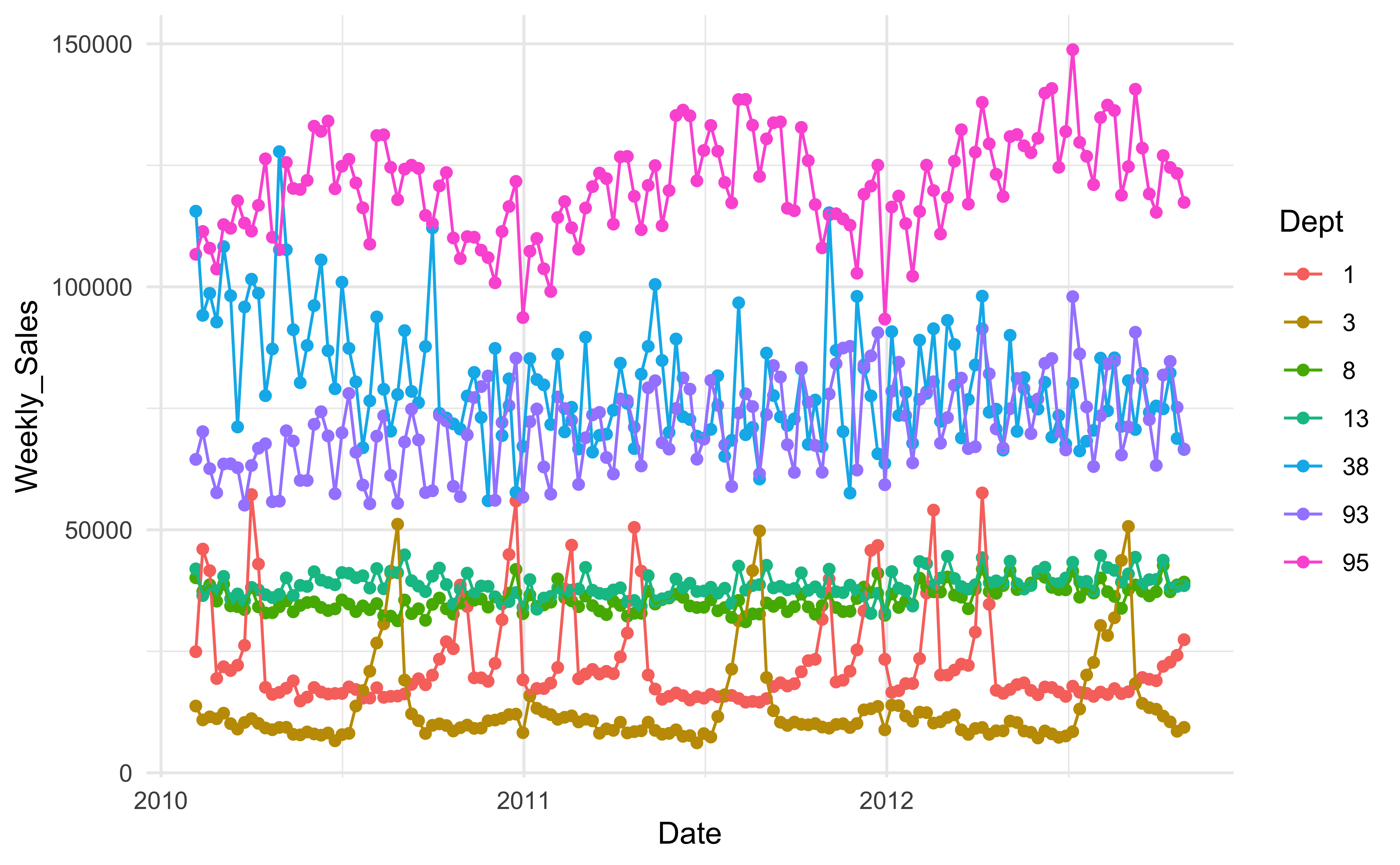

For more analysis and forecasting etc., it is useful to convert this tibble into a tsibble:

walmart_tsibble <- as_tsibble(walmart_sales_weekly,
  index = Date,
  key = c(id, Dept)
)
walmart_tsibble

ABCDEFGHIJ0123456789

id <fct>	Store <dbl>	Dept <dbl>	Date <date>	Weekly_Sales <dbl>	IsHoliday <lgl>	Type <chr>	Size <dbl>	Temperature <dbl>	Fuel_Price <dbl>
1_1	1	1	2010-02-05	24924.50	FALSE	A	151315	42.31	2.572
1_1	1	1	2010-02-12	46039.49	TRUE	A	151315	38.51	2.548
1_1	1	1	2010-02-19	41595.55	FALSE	A	151315	39.93	2.514
1_1	1	1	2010-02-26	19403.54	FALSE	A	151315	46.63	2.561
1_1	1	1	2010-03-05	21827.90	FALSE	A	151315	46.50	2.625
1_1	1	1	2010-03-12	21043.39	FALSE	A	151315	57.79	2.667
1_1	1	1	2010-03-19	22136.64	FALSE	A	151315	54.58	2.720
1_1	1	1	2010-03-26	26229.21	FALSE	A	151315	51.45	2.732
1_1	1	1	2010-04-02	57258.43	FALSE	A	151315	62.27	2.719
1_1	1	1	2010-04-09	42960.91	FALSE	A	151315	65.86	2.770

The 7D states the data is weekly. There is a Date column and all the other numerical variables are time-varying quantities. The categorical variables such as id, and Dept allow us to identify separate time series in the data, and these have 7 combinations hence are 7 time series in this data, as indicated.

Let us plot Weekly_Sales, colouring the time series by Dept:

walmart_tsibble %>%
  gf_line(Weekly_Sales ~ Date,
    colour = ~ as_factor(Dept), data = .
  ) %>%
  gf_point() %>%
  gf_theme(theme_minimal()) %>%
  labs(title = "Weekly Sales by Dept at Walmart")

[[1]]


$title
[1] "Weekly Sales by Dept at Walmart"

attr(,"class")
[1] "labels"

We can also do a quick autoplot that seems to offer less control and is also not interactive.

walmart_tsibble %>%
  dplyr::group_by(Dept) %>%
  autoplot(Weekly_Sales) %>%
  gf_theme(theme_minimal())

`tsibble` format data

In the packages tsibbledata and fpp3 we have a good choice of tsibble format data. Let us pick one:

hh_budget

ABCDEFGHIJ0123456789

Country <chr>	Year <dbl>	Debt <dbl>	DI <dbl>	Expenditure <dbl>	Savings <dbl>	Wealth <dbl>	Unemployment <dbl>
Australia	1995	95.68999	3.71954533	3.40431125	5.2389216	314.9344	8.472281
Australia	1996	99.53078	3.98447837	2.97174126	6.4716693	314.5559	8.506114
Australia	1997	107.54020	2.51634483	4.94912455	3.7399359	323.2357	8.362488
Australia	1998	114.63320	4.02375433	5.73154083	1.2875994	339.3139	7.677429
Australia	1999	121.09980	3.84019750	4.25782877	0.6377422	354.4382	6.873791
Australia	2000	126.42540	3.76981375	3.18030349	1.9904011	350.2795	6.285546
Australia	2001	132.01050	4.36426631	3.09770520	3.2373997	347.8053	6.742173
Australia	2002	149.09440	0.02182040	4.03171701	-1.1518200	348.7379	6.368911
Australia	2003	159.24950	6.05659181	5.03899495	-0.4134631	359.9007	5.928420
Australia	2004	169.58480	5.52682017	4.54493368	0.6568372	378.5653	5.396734

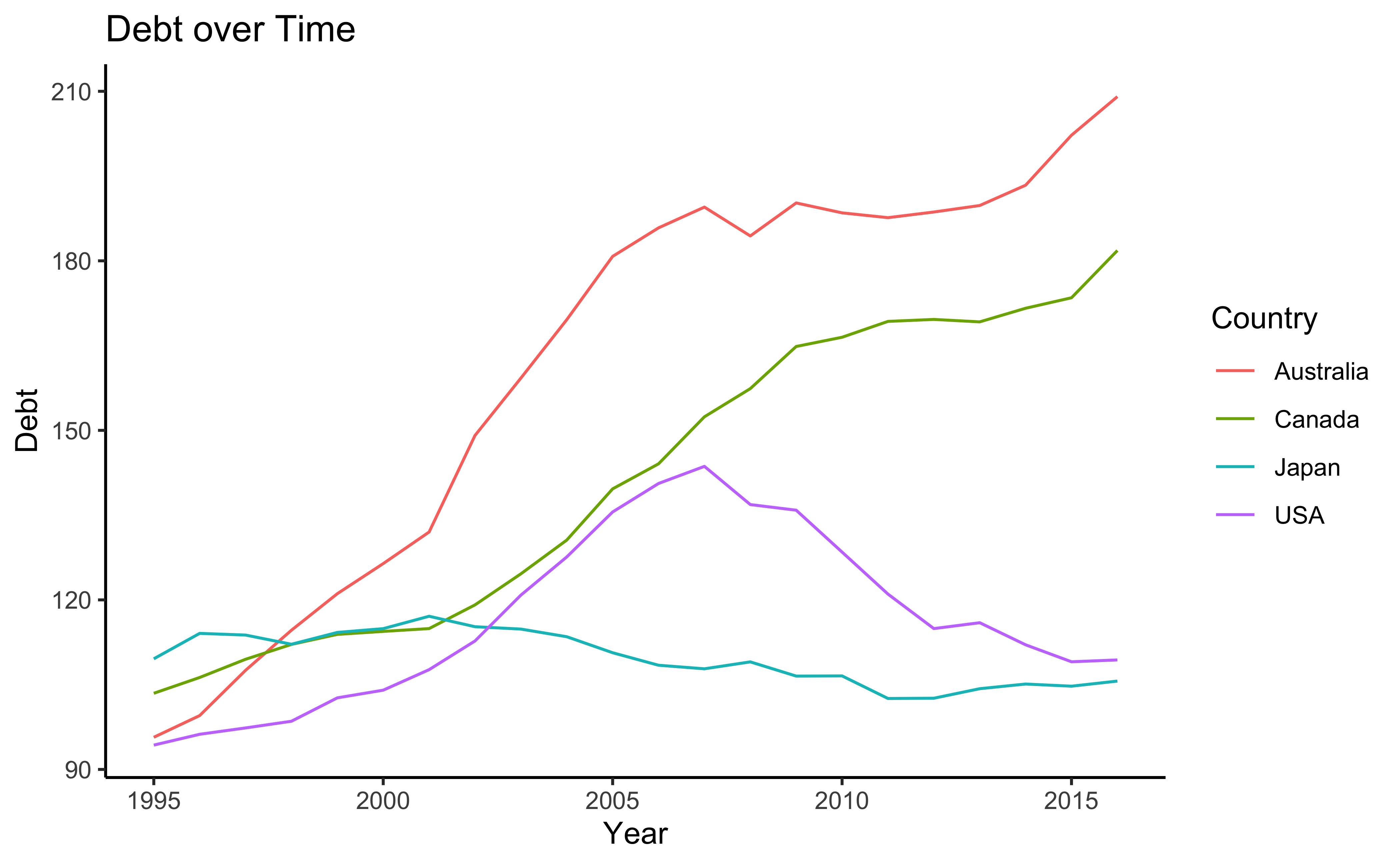
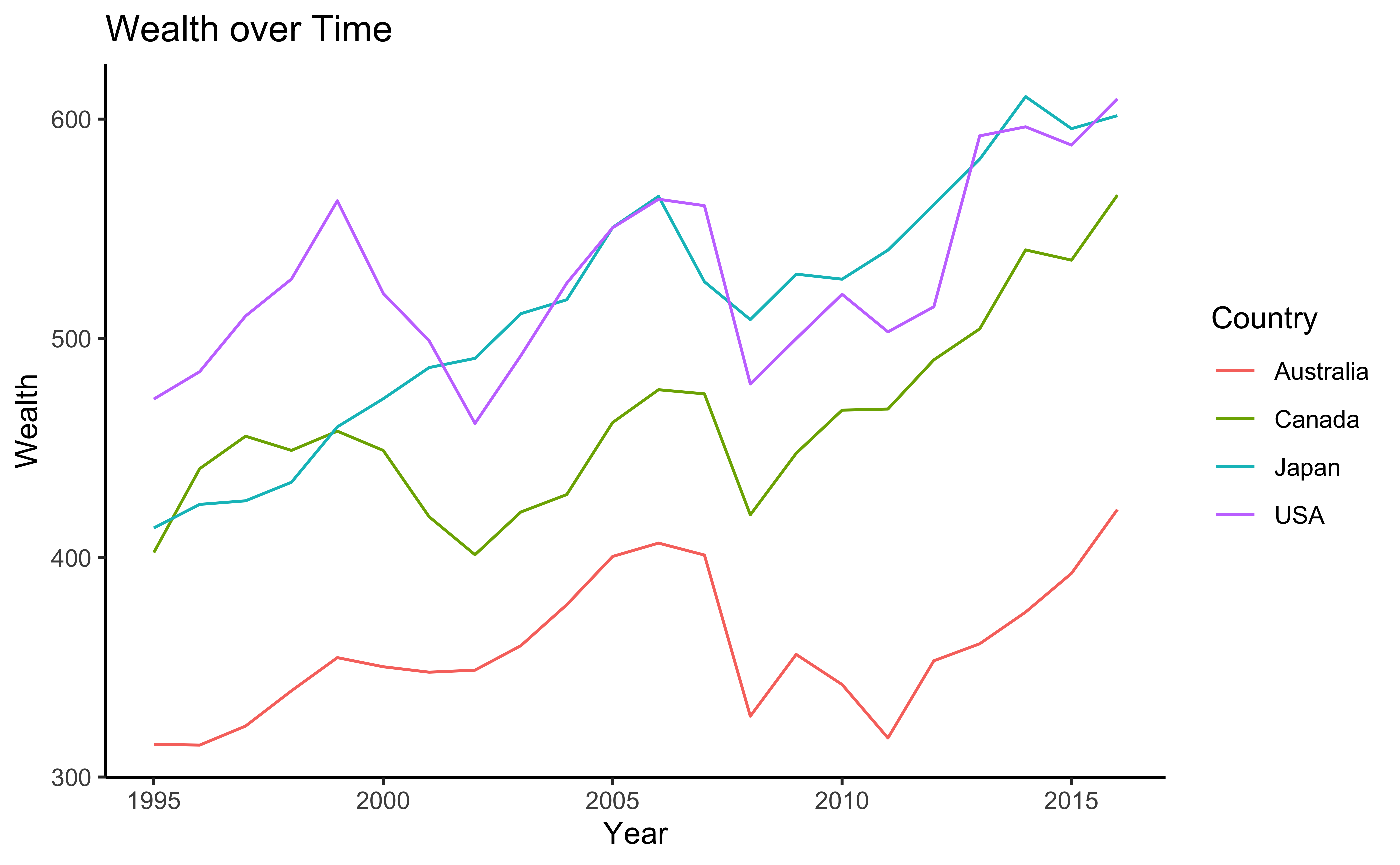
There are 4 keys ( id variables ) here, one for each country. Six other quantitative columns are the individual series. Let us plot (some of) the timeseries:

ggplot2::theme_set(theme_classic())
hh_budget %>%
  gf_path(Debt ~ Year,
    colour = ~Country,
    title = "Debt over Time"
  )
##
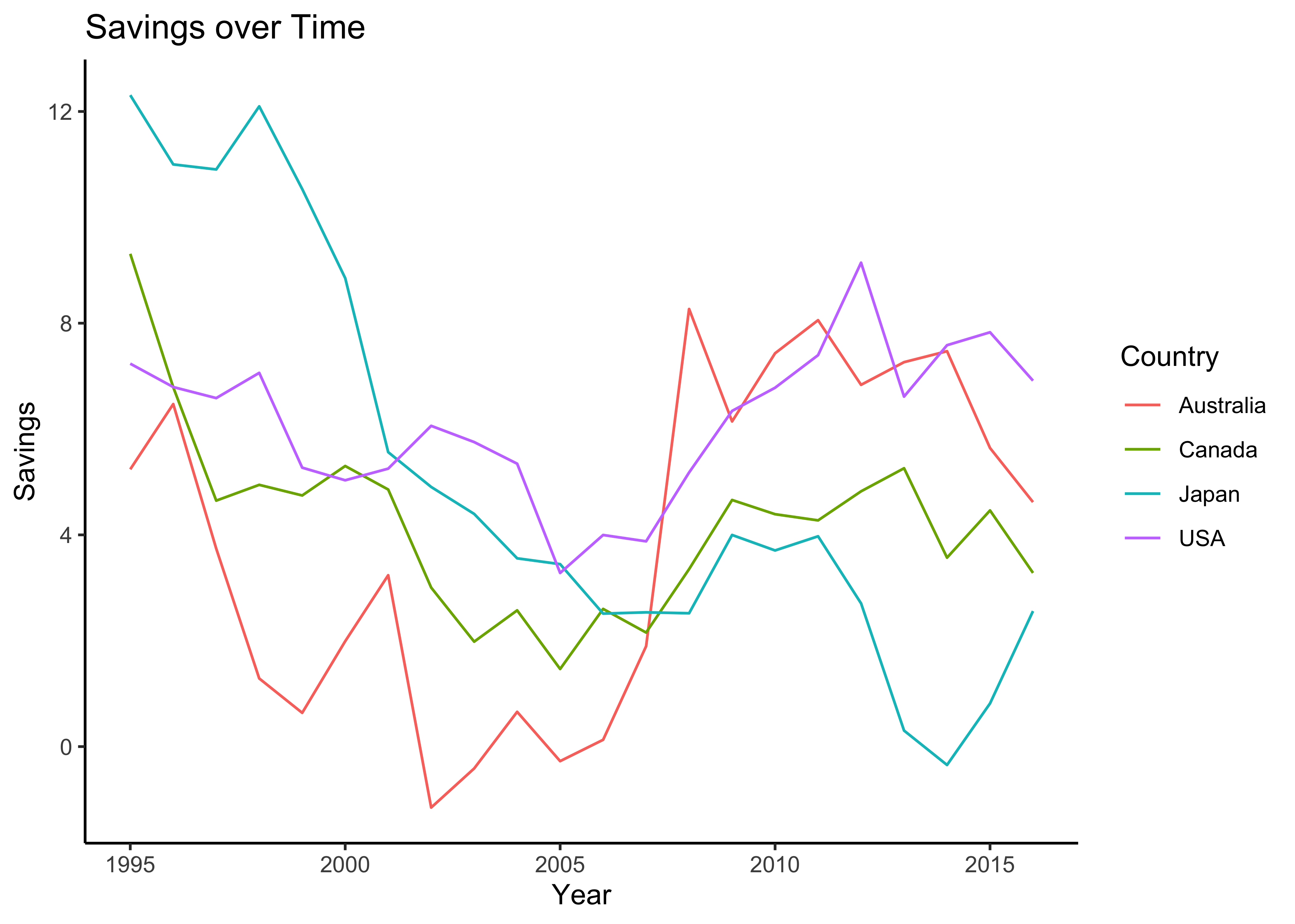
hh_budget %>%
  gf_path(Savings ~ Year,
    colour = ~Country,
    title = "Savings over Time"
  )
##
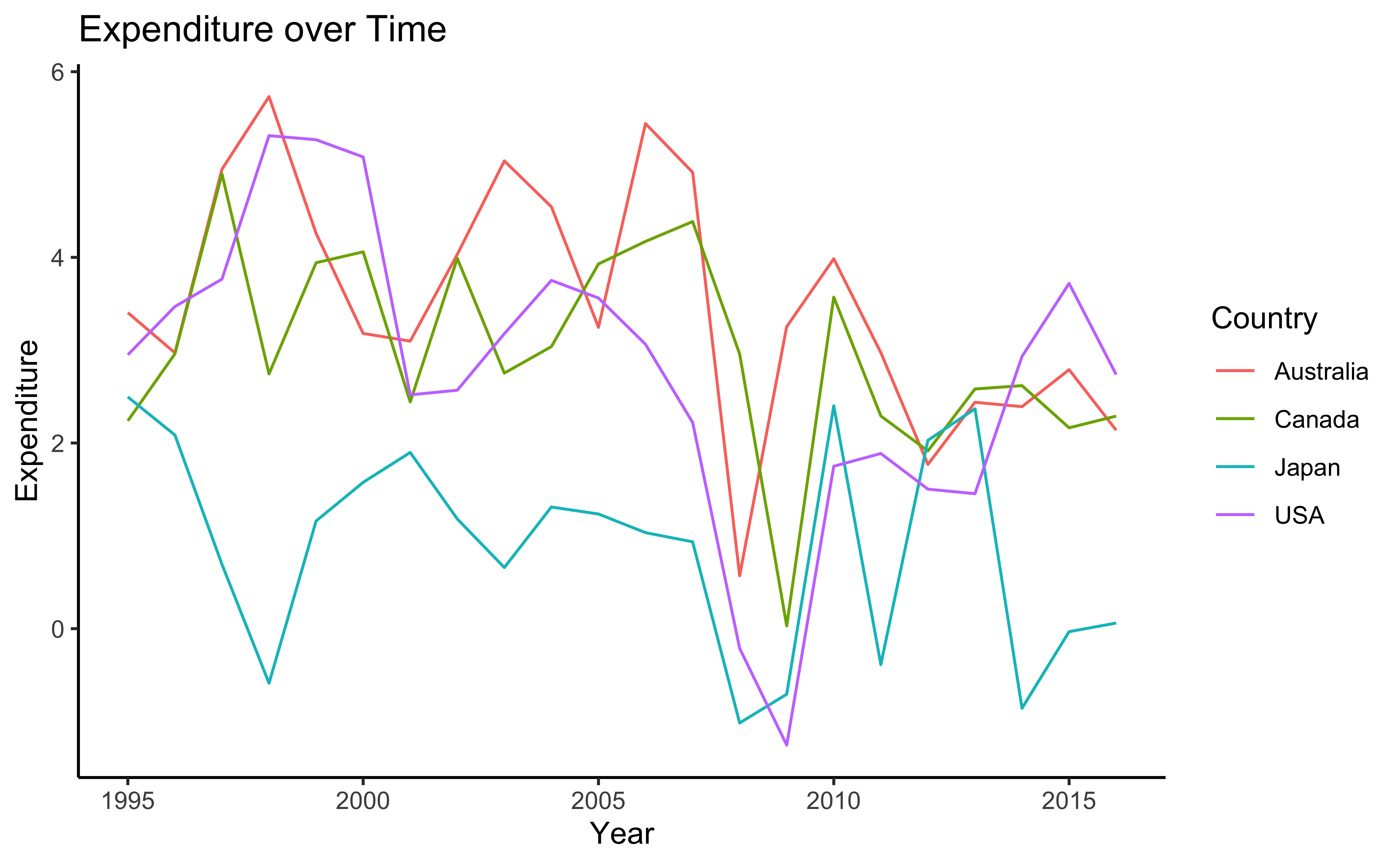
hh_budget %>%
  gf_path(Expenditure ~ Year,
    colour = ~Country,
    title = "Expenditure over Time"
  )
##
hh_budget %>%
  gf_path(Wealth ~ Year,
    colour = ~Country,
    title = "Wealth over Time"
  )

One more example

Often we have data in table form, that is time-oriented, with a date like column, and we need to convert it into a tsibble for analysis:

prison <- readr::read_csv("https://OTexts.com/fpp3/extrafiles/prison_population.csv")
glimpse(prison)

Rows: 3,072
Columns: 6
$ Date       <date> 2005-03-01, 2005-03-01, 2005-03-01, 2005-03-01, 2005-03-01…
$ State      <chr> "ACT", "ACT", "ACT", "ACT", "ACT", "ACT", "ACT", "ACT", "NS…
$ Gender     <chr> "Female", "Female", "Female", "Female", "Male", "Male", "Ma…
$ Legal      <chr> "Remanded", "Remanded", "Sentenced", "Sentenced", "Remanded…
$ Indigenous <chr> "ATSI", "Non-ATSI", "ATSI", "Non-ATSI", "ATSI", "Non-ATSI",…
$ Count      <dbl> 0, 2, 0, 5, 7, 58, 5, 101, 51, 131, 145, 323, 355, 1617, 12…

We have a Date column for the time index, and we have unique key variables like State, Gender, Legal and Indigenous. Count is the value that is variable over time. It also appears that the data is quarterly, since mosaic::inspect reports the max_diff in the Date column as $92$ . .

Run mosaic::inspect(prison) in your Console

prison_tsibble <- prison %>%
  mutate(quarter = yearquarter(Date)) %>%
  select(-Date) %>% # Remove the Date column now that we have quarters
  as_tsibble(index = quarter, key = c(State, Gender, Legal, Indigenous))

prison_tsibble

ABCDEFGHIJ0123456789

State <chr>	Gender <chr>	Legal <chr>	Indigenous <chr>	Count <dbl>	quarter <qtr>
ACT	Female	Remanded	ATSI	0	2005 Q1
ACT	Female	Remanded	ATSI	1	2005 Q2
ACT	Female	Remanded	ATSI	0	2005 Q3
ACT	Female	Remanded	ATSI	0	2005 Q4
ACT	Female	Remanded	ATSI	1	2006 Q1
ACT	Female	Remanded	ATSI	1	2006 Q2
ACT	Female	Remanded	ATSI	1	2006 Q3
ACT	Female	Remanded	ATSI	0	2006 Q4
ACT	Female	Remanded	ATSI	0	2007 Q1
ACT	Female	Remanded	ATSI	1	2007 Q2

(Here, ATSI stands for Aboriginal or Torres Strait Islander.). We have $64$ time series here, organized quarterly.

Let us examine the key variables:

prison_tsibble %>% distinct(Indigenous)

ABCDEFGHIJ0123456789

Indigenous <chr>
ATSI
Non-ATSI

prison_tsibble %>% distinct(State)

ABCDEFGHIJ0123456789

State <chr>
ACT
NSW
NT
QLD
SA
TAS
VIC
WA

So we can plot the time series, faceted / coloured by State:

prison_tsibble %>%
  tsibble::index_by() %>%
  group_by(Indigenous, State) %>%
  # filter(State == "NSW") %>%
  summarise(Total = sum(Count)) %>%
  gf_point(Total ~ quarter,
    colour = ~Indigenous,
    shape = ~Indigenous
  ) %>%
  gf_line() %>%
  # Note that the y-axes are all. different!!
  gf_facet_wrap(vars(State), scale = "free_y") %>%
  gf_theme(theme_minimal())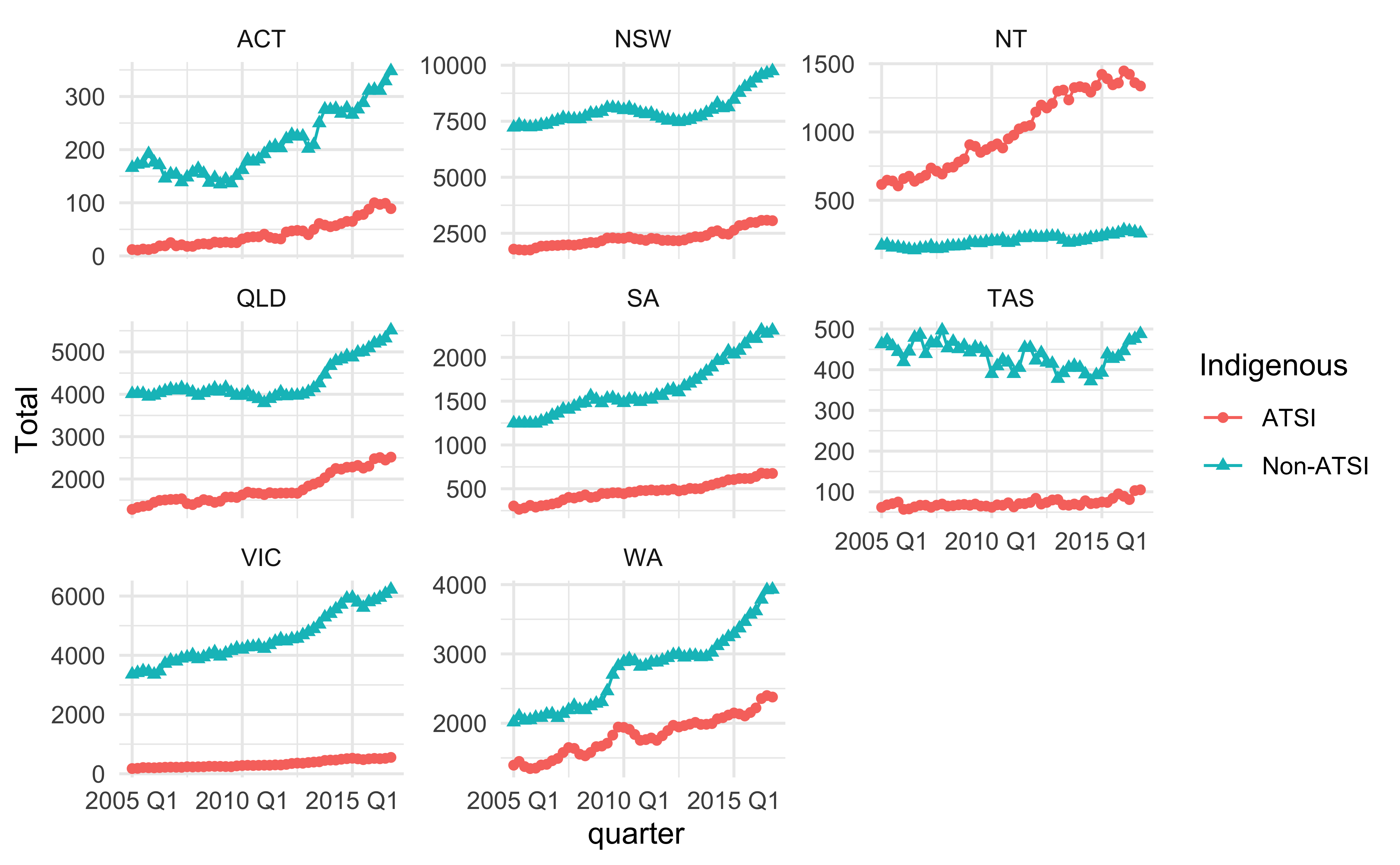

Hmm…looks like New South Wales(NSW) as something different going on compared to the rest of the states in Aus. Because of the large cities there…

Decomposing Time Series

We can decompose the Weekly_Sales into components representing trends, seasonal events that repeat, and irregular noise. Since each Dept could have a different set of trends, we will do this first for one Dept, say Dept #95:

walmart_decomposed_season <- walmart_tsibble %>%
  dplyr::filter(Dept == "95") %>% # filter for Dept 95
  #
  # feasts depends upon fabletools.
  #
  fabletools::model(
    season = STL(Weekly_Sales ~ season(window = "periodic"))
  )
walmart_decomposed_season %>% fabletools::components()

ABCDEFGHIJ0123456789

id <fct>	Dept <dbl>	.model <chr>	Date <date>	Weekly_Sales <dbl>	trend <dbl>	season_year <dbl>	remainder <dbl>	season_adjust <dbl>
1_95	95	season	2010-02-05	106690.06	113713.4	-6508.1600	-515.21431	113198.22
1_95	95	season	2010-02-12	111390.36	113802.0	-729.1725	-1682.49225	112119.53
1_95	95	season	2010-02-19	107952.07	113890.6	-729.1726	-5209.37273	108681.24
1_95	95	season	2010-02-26	103652.58	113979.2	-729.1726	-9597.45320	104381.75
1_95	95	season	2010-03-05	112807.75	114067.8	-5470.6885	4210.64214	118278.44
1_95	95	season	2010-03-12	112048.41	114156.4	-5470.6885	3362.71165	117519.10
1_95	95	season	2010-03-19	117716.13	114245.0	-5470.6885	8941.84115	123186.82
1_95	95	season	2010-03-26	113117.35	114333.6	-11414.6478	10198.42988	124532.00
1_95	95	season	2010-04-02	111466.37	114422.2	-11414.6478	8458.85933	122881.02
1_95	95	season	2010-04-09	116770.82	114509.5	-11414.6477	13675.94797	128185.47

###
walmart_decomposed_ets <- walmart_tsibble %>%
  dplyr::filter(Dept == "95") %>% # filter for Dept 95
  #
  # feasts depends upon fabletools.
  #
  fabletools::model(
    ets = ETS(box_cox(Weekly_Sales, 0.3))
  )
###
walmart_decomposed_ets %>% fabletools::components()

ABCDEFGHIJ0123456789

id <fct>	Dept <dbl>	.model <chr>	Date <date>	box_cox(Weekly_Sales, 0.3) <dbl>	level <dbl>	remainder <dbl>
1_95	95	ets	2010-01-29	NA	104.9244	NA
1_95	95	ets	2010-02-05	104.14377	104.6896	-0.780651335
1_95	95	ets	2010-02-12	105.54288	104.9463	0.853307155
1_95	95	ets	2010-02-19	104.52359	104.8191	-0.422680545
1_95	95	ets	2010-02-26	103.21650	104.3370	-1.602619221
1_95	95	ets	2010-03-05	105.95667	104.8242	1.619652467
1_95	95	ets	2010-03-12	105.73545	105.0984	0.911201935
1_95	95	ets	2010-03-19	107.36206	105.7793	2.263701564
1_95	95	ets	2010-03-26	106.04656	105.8597	0.267232522
1_95	95	ets	2010-04-02	105.56517	105.7711	-0.294553642

###
walmart_decomposed_arima <- walmart_tsibble %>%
  dplyr::filter(Dept == "95") %>% # filter for Dept 95
  fabletools::model(arima = ARIMA(log(Weekly_Sales)))
walmart_decomposed_arima %>% broom::tidy()

ABCDEFGHIJ0123456789

id <fct>	Dept <dbl>	.model <chr>	term <chr>	estimate <dbl>	std.error <dbl>	statistic <dbl>	p.value <dbl>
1_95	95	arima	ar1	-0.1483206	0.12573909	-1.179590	2.401357e-01
1_95	95	arima	ar2	-0.8286585	0.03745076	-22.126613	7.264053e-48
1_95	95	arima	ar3	-0.3856024	0.10496648	-3.673576	3.380457e-04
1_95	95	arima	ma1	-0.4641933	0.11752561	-3.949721	1.227609e-04
1_95	95	arima	ma2	0.6758916	0.08334419	8.109643	2.153610e-13

walmart_decomposed_season %>%
  components() %>%
  autoplot() +
  labs(title = "Seasonal Variations in Weekly Sales, Dept #95")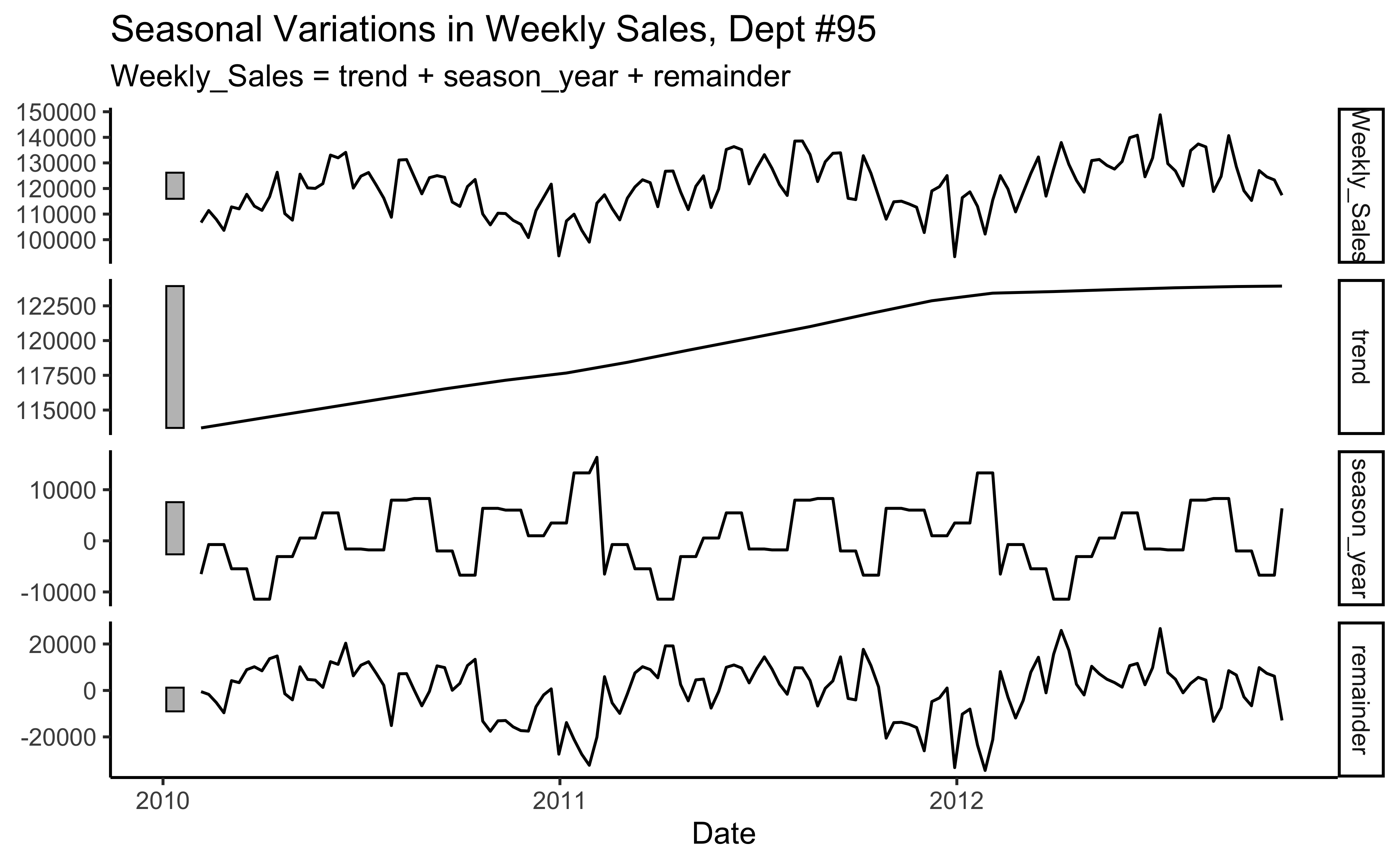

walmart_decomposed_ets %>%
  components() %>%
  autoplot() +
  labs(title = "ETS Variations in Weekly Sales, Dept #95")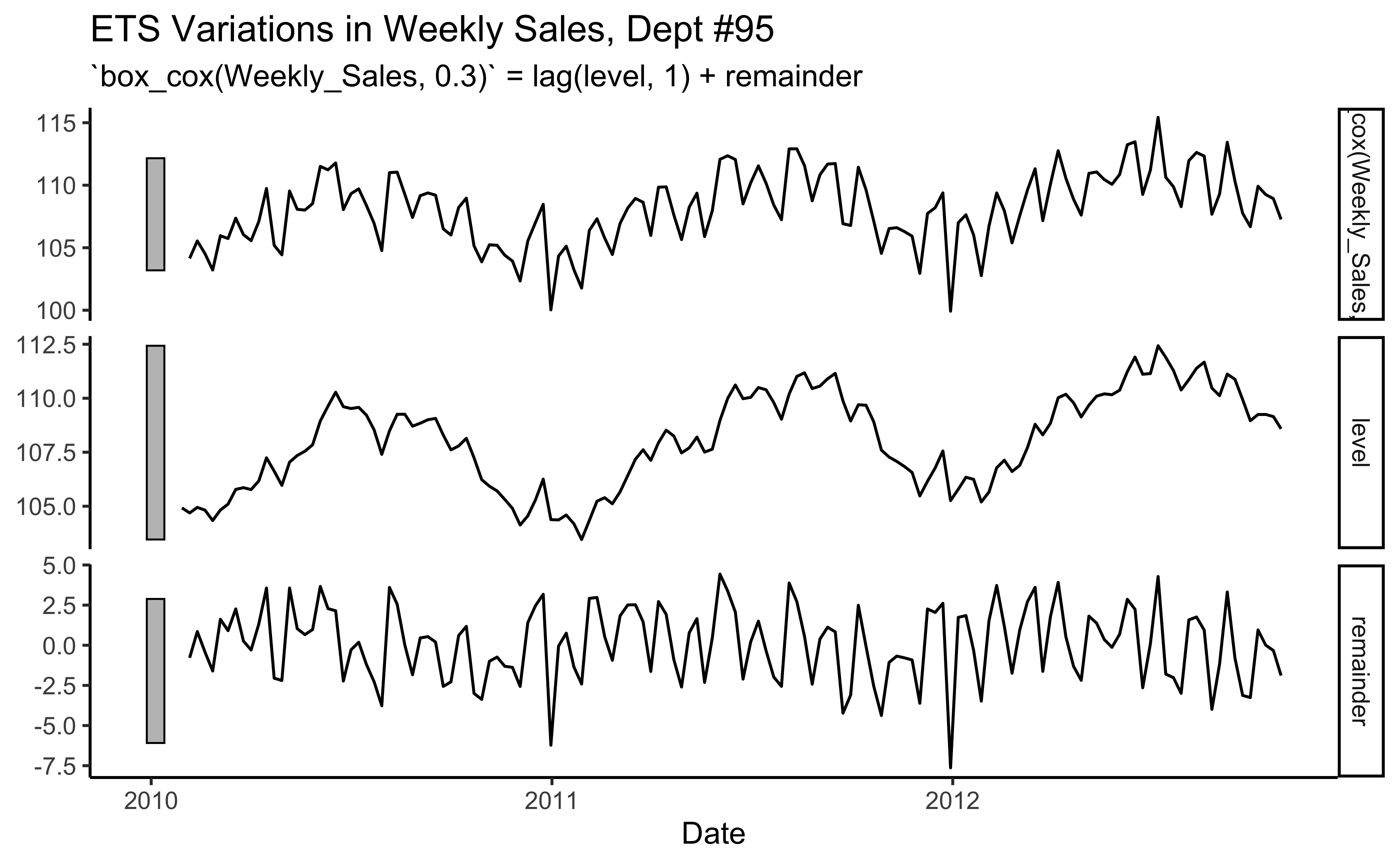

Conclusion

TBW

References

Forecasting: Principles and Practice (3rd ed) Rob J Hyndman and George Athanasopoulos

Introduction

Introduction to Time Series: Data Formats

Creating time series

ts format data

tibble format data

tsibble format data

One more example

Decomposing Time Series

Conclusion

References

`ts` format data

`tibble` format data

`tsibble` format data