Grain Transportation Cartels
Setting up R Packages
Plot Theme
Show the Code
# https://stackoverflow.com/questions/74491138/ggplot-custom-fonts-not-working-in-quarto

# Chunk options
knitr::opts_chunk$set(
  fig.width = 7,
  fig.asp = 0.618, # Golden Ratio
  # out.width = "80%",
  fig.align = "center"
)
### Ggplot Theme
### https://rpubs.com/mclaire19/ggplot2-custom-themes

theme_custom <- function() {
  font <- "Roboto Condensed" # assign font family up front

  theme_classic(base_size = 14) %+replace% # replace elements we want to change

    theme(
      panel.grid.minor = element_blank(), # strip minor gridlines
      text = element_text(family = font),
      # text elements
      plot.title = element_text( # title
        family = font, # set font family
        size = 16, # set font size
        face = "bold", # bold typeface
        hjust = 0, # left align
        # vjust = 2                #raise slightly
        margin = margin(0, 0, 10, 0)
      ),
      plot.subtitle = element_text( # subtitle
        family = font, # font family
        size = 14, # font size
        hjust = 0,
        margin = margin(2, 0, 5, 0)
      ),
      plot.caption = element_text( # caption
        family = font, # font family
        size = 8, # font size
        hjust = 1
      ), # right align

      axis.title = element_text( # axis titles
        family = font, # font family
        size = 10 # font size
      ),
      axis.text = element_text( # axis text
        family = font, # axis family
        size = 8
      ) # font size
    )
}

# Set graph theme
theme_set(new = theme_custom())
#
Introduction
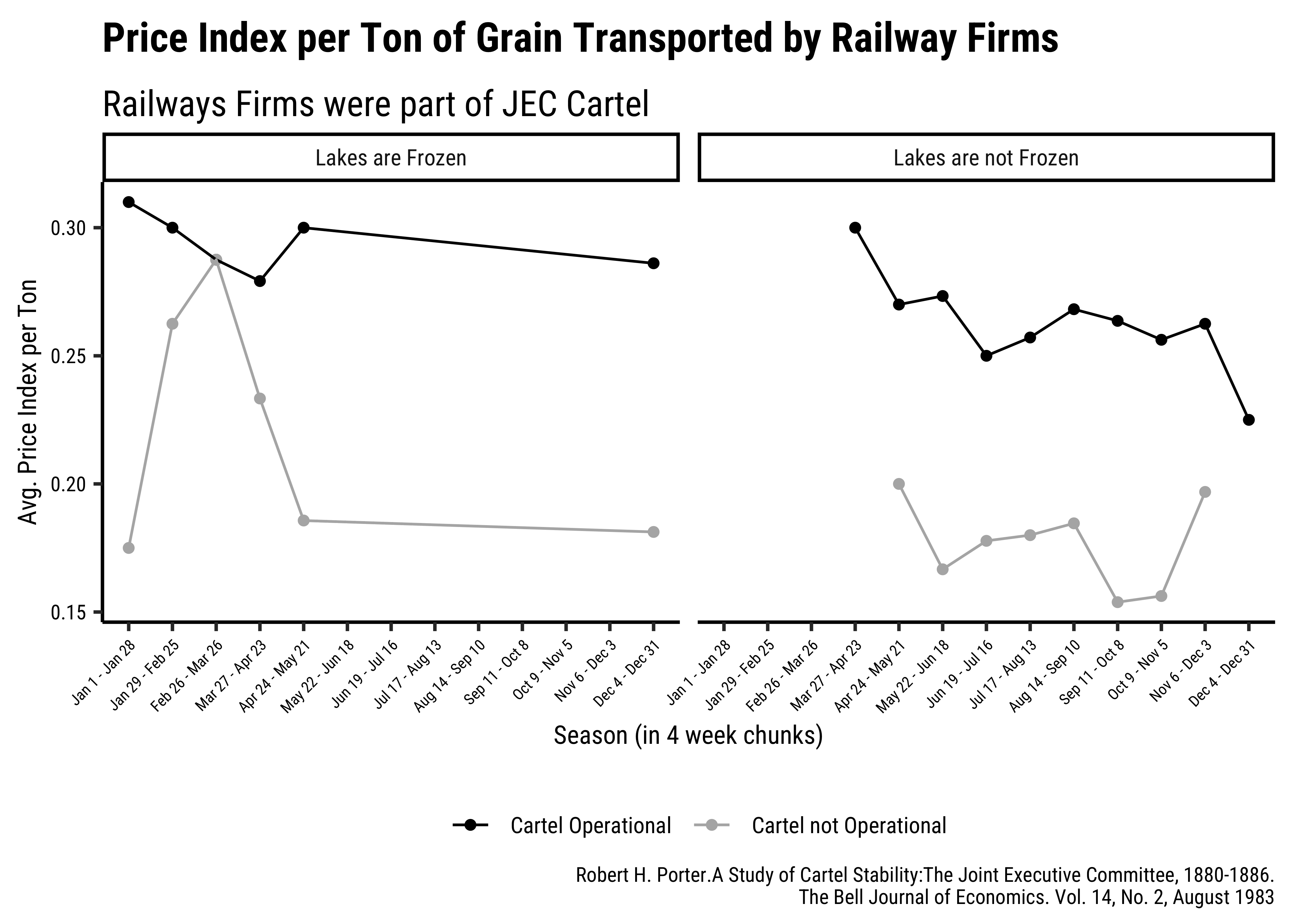
From: Robert H. Porter (1983). A Study of Cartel Stability: The Joint Executive Committee, 1880-1886. The Bell Journal of Economics, Vol. 14, No. 2 (Autumn, 1983), pp. 301-314:
The Joint Executive Committee (JEC) was a cartel (of railroad firms) which controlled eastbound freight shipments from Chicago to the Atlantic seaboard in the 1880’s. While different railroad firms in the JEC shipped grain to different port cities (for example, Baltimore and New York), most of the wheat handled by the cartel was subsequently exported overseas, and the rates charged by different firms (were) adjusted to compensate for differences in ocean shipping rates.
Prices, rather than quantity, has typically been thought to be the strategic variable of firms in the rail-freight industry. Total demand was quite variable, and so the actual market share of any particular railroad firm would depend on both the prices charged by all the firms as well as unpredictable (random) forces. Price wars were not random, but precipitated by periods of slackened demand, which were presumably unpredictable, at least to some extent.
On the other hand, the predictable fluctuations in demand that resulted from the annual opening and closing of the Great Lakes (Superior / Michigan / Huron / Ontario / Erie ) to shipping (because they were frozen in winter), which determined the degree of outside competition, did not disrupt industry conduct. Rather, rates adjusted systematically with the lake navigation season.
This dataset is available on Vincent Arel-Bundock’s dataset repository, and is part of the R package AER (Applied Econometrics in R).
Read the Data
cartelstability <- read_csv("https://vincentarelbundock.github.io/Rdatasets/csv/AER/CartelStability.csv")
cartelstabilityrownames <dbl> | price <dbl> | cartel <chr> | quantity <dbl> | season <chr> | ice <chr> |
|---|---|---|---|---|---|
| 1 | 0.400 | yes | 13632 | Jan 1 - Jan 28 | yes |
| 2 | 0.400 | yes | 20035 | Jan 1 - Jan 28 | yes |
| 3 | 0.400 | yes | 16319 | Jan 1 - Jan 28 | yes |
| 4 | 0.400 | yes | 12603 | Jan 1 - Jan 28 | yes |
| 5 | 0.400 | yes | 23079 | Jan 29 - Feb 25 | yes |
| 6 | 0.400 | yes | 19652 | Jan 29 - Feb 25 | yes |
| 7 | 0.400 | yes | 16211 | Jan 29 - Feb 25 | yes |
| 8 | 0.400 | yes | 22914 | Jan 29 - Feb 25 | yes |
| 9 | 0.400 | yes | 23710 | Feb 26 - Mar 26 | yes |
| 10 | 0.350 | yes | 23036 | Feb 26 - Mar 26 | yes |
glimpse(cartelstability)Rows: 328
Columns: 6
$ rownames <dbl> 1, 2, 3, 4, 5, 6, 7, 8, 9, 10, 11, 12, 13, 14, 15, 16, 17, 18…
$ price <dbl> 0.40, 0.40, 0.40, 0.40, 0.40, 0.40, 0.40, 0.40, 0.40, 0.35, 0…
$ cartel <chr> "yes", "yes", "yes", "yes", "yes", "yes", "yes", "yes", "yes"…
$ quantity <dbl> 13632, 20035, 16319, 12603, 23079, 19652, 16211, 22914, 23710…
$ season <chr> "Jan 1 - Jan 28", "Jan 1 - Jan 28", "Jan 1 - Jan 28", "Jan…
$ ice <chr> "yes", "yes", "yes", "yes", "yes", "yes", "yes", "yes", "yes"…Data Dictionary
Write in.
Write in.
Write in.
Research Question
How do prices for per-tonne grain transport vary based on whether the cartel is working or not? Does this depend upon whether it is summer time or winter time? Why?
Inspect/Analyse/Transform the Data
```{r}
#| label: data-preprocessing
#
# Write in your code here
# to prepare this data as shown below
# to generate the plot that follows
# Rename Variables if needed
# Change data to factors etc.
# Set up Counts, histograms etc
```rownames <dbl> | price <dbl> | cartel <fct> | quantity <dbl> | season <ord> | ice <fct> |
|---|---|---|---|---|---|
| 1 | 0.400 | Cartel Operational | 13632 | Jan 1 - Jan 28 | Lakes are Frozen |
| 2 | 0.400 | Cartel Operational | 20035 | Jan 1 - Jan 28 | Lakes are Frozen |
| 3 | 0.400 | Cartel Operational | 16319 | Jan 1 - Jan 28 | Lakes are Frozen |
| 4 | 0.400 | Cartel Operational | 12603 | Jan 1 - Jan 28 | Lakes are Frozen |
| 5 | 0.400 | Cartel Operational | 23079 | Jan 29 - Feb 25 | Lakes are Frozen |
| 6 | 0.400 | Cartel Operational | 19652 | Jan 29 - Feb 25 | Lakes are Frozen |
| 7 | 0.400 | Cartel Operational | 16211 | Jan 29 - Feb 25 | Lakes are Frozen |
| 8 | 0.400 | Cartel Operational | 22914 | Jan 29 - Feb 25 | Lakes are Frozen |
| 9 | 0.400 | Cartel Operational | 23710 | Feb 26 - Mar 26 | Lakes are Frozen |
| 10 | 0.350 | Cartel Operational | 23036 | Feb 26 - Mar 26 | Lakes are Frozen |
Some summarizing…
season <ord> | cartel <fct> | ice <fct> | avg_price <dbl> | mean_tonnage <dbl> |
|---|---|---|---|---|
| Jan 1 - Jan 28 | Cartel Operational | Lakes are Frozen | 0.3100000 | 23461.90 |
| Jan 1 - Jan 28 | Cartel not Operational | Lakes are Frozen | 0.1750000 | 27646.12 |
| Jan 29 - Feb 25 | Cartel Operational | Lakes are Frozen | 0.3000000 | 30157.60 |
| Jan 29 - Feb 25 | Cartel not Operational | Lakes are Frozen | 0.2625000 | 23731.00 |
| Feb 26 - Mar 26 | Cartel Operational | Lakes are Frozen | 0.2875000 | 28736.44 |
| Feb 26 - Mar 26 | Cartel not Operational | Lakes are Frozen | 0.2875000 | 29584.58 |
| Mar 27 - Apr 23 | Cartel Operational | Lakes are Frozen | 0.2791667 | 24984.75 |
| Mar 27 - Apr 23 | Cartel Operational | Lakes are not Frozen | 0.3000000 | 23799.25 |
| Mar 27 - Apr 23 | Cartel not Operational | Lakes are Frozen | 0.2333333 | 46858.83 |
| Apr 24 - May 21 | Cartel Operational | Lakes are Frozen | 0.3000000 | 36457.33 |
Plot the Data
Task and Discussion
- Complete the Data Dictionary.
- Select and Transform the variables as shown.
- Create the graphs shown and discuss the following questions:
- Identify the type of charts
- Identify the variables used for various geometrical aspects (x, y, fill…). Name the variables appropriately.
- What research activity might have been carried out to obtain the data graphed here? Provide some details.
- What pre-processing of the data was required to create the chart?
- Explain what happens when it is stated “cartel is working” and “cartel is not working”.
- How do prices for per-tonne grain transport vary based on whether the cartel is working or not? Does this depend upon whether it is summer time or winter time? Why?
- Is the cartel beneficial for customers of the JEC? What would be their behaviour based on whether the cartel was operational or not?