Movie Profits

Setting up R Packages

library(tidyverse)
library(mosaic)
library(skimr)
library(ggformula)

Plot Theme and Fonts

Show the Code

```{r}
#| code-fold: true
#| message: false
#| warning: false

knitr::opts_chunk$set(
  fig.width = 7,
  fig.asp = 0.618, # Golden Ratio
  # out.width = "80%",
  fig.align = "center"
)
##
## https://stackoverflow.com/questions/36476751/associate-a-color-palette-with-ggplot2-theme
##
my_colours <- c("#fd7f6f", "#7eb0d5", "#b2e061", "#bd7ebe", "#ffb55a", "#ffee65", "#beb9db", "#fdcce5", "#8bd3c7")
my_pastels <- c("#66C5CC", "#F6CF71", "#F89C74", "#DCB0F2", "#87C55F", "#9EB9F3", "#FE88B1", "#C9DB74", "#8BE0A4", "#B497E7", "#D3B484", "#B3B3B3")
my_greys <- c("#000000", "#333333", "#666666", "#999999", "#cccccc")
my_vivids <- c("#E58606", "#5D69B1", "#52BCA3", "#99C945", "#CC61B0", "#24796C", "#DAA51B", "#2F8AC4", "#764E9F", "#ED645A", "#CC3A8E", "#A5AA99")

my_bolds <- c("#7F3C8D", "#11A579", "#3969AC", "#F2B701", "#E73F74", "#80BA5A", "#E68310", "#008695", "#CF1C90", "#f97b72", "#4b4b8f", "#A5AA99")

library(systemfonts)
library(showtext)
## Clean the slate
systemfonts::clear_local_fonts()
systemfonts::clear_registry()
##
showtext_opts(dpi = 96) # set DPI for showtext
sysfonts::font_add(
  family = "Alegreya",
  regular = "../../../../../../fonts/Alegreya-Regular.ttf",
  bold = "../../../../../../fonts/Alegreya-Bold.ttf",
  italic = "../../../../../../fonts/Alegreya-Italic.ttf",
  bolditalic = "../../../../../../fonts/Alegreya-BoldItalic.ttf"
)

sysfonts::font_add(
  family = "Roboto Condensed",
  regular = "../../../../../../fonts/RobotoCondensed-Regular.ttf",
  bold = "../../../../../../fonts/RobotoCondensed-Bold.ttf",
  italic = "../../../../../../fonts/RobotoCondensed-Italic.ttf",
  bolditalic = "../../../../../../fonts/RobotoCondensed-BoldItalic.ttf"
)
showtext_auto(enable = TRUE) # enable showtext
##
theme_custom <- function() {
  font <- "Alegreya" # assign font family up front

  theme_classic(base_size = 14, base_family = font) %+replace% # replace elements we want to change

    theme(
      text = element_text(family = font), # set base font family

      # text elements
      plot.title = element_text( # title
        family = font, # set font family
        size = 24, # set font size
        face = "bold", # bold typeface
        hjust = 0, # left align
        margin = margin(t = 5, r = 0, b = 5, l = 0)
      ), # margin
      plot.title.position = "plot",
      plot.subtitle = element_text( # subtitle
        family = font, # font family
        size = 14, # font size
        hjust = 0, # left align
        margin = margin(t = 5, r = 0, b = 10, l = 0)
      ), # margin

      plot.caption = element_text( # caption
        family = font, # font family
        size = 9, # font size
        hjust = 1
      ), # right align

      plot.caption.position = "plot", # right align

      plot.background = element_rect(fill = "navajowhite"),
      axis.title = element_text( # axis titles
        family = "Roboto Condensed", # font family
        size = 12
      ), # font size

      axis.text = element_text( # axis text
        family = "Roboto Condensed", # font family
        size = 9
      ), # font size

      axis.text.x = element_text( # margin for axis text
        margin = margin(5, b = 10)
      )

      # since the legend often requires manual tweaking
      # based on plot content, don't define it here
    )
}

## Use available fonts in ggplot text geoms too!
update_geom_defaults(geom = "text", new = list(
  family = "Roboto Condensed",
  face = "plain",
  size = 3.5,
  color = "#2b2b2b"
))

## Set the theme
theme_set(new = theme_custom())
```

Introduction

This is a dataset pertaining to movies and genres, modified for ease of analysis and plotting.

Data

Error in movie_profit_raw %>% select(-...1) %>% dplyr::mutate(release_date = as.Date(parse_date_time(release_date, : could not find function "%>%"

Error: object 'movie_profit' not found

Download the Modified data

Data Dictionary

Quantitative Variables

Write in.

Qualitative Variables

Write in.

Observations

Write in.

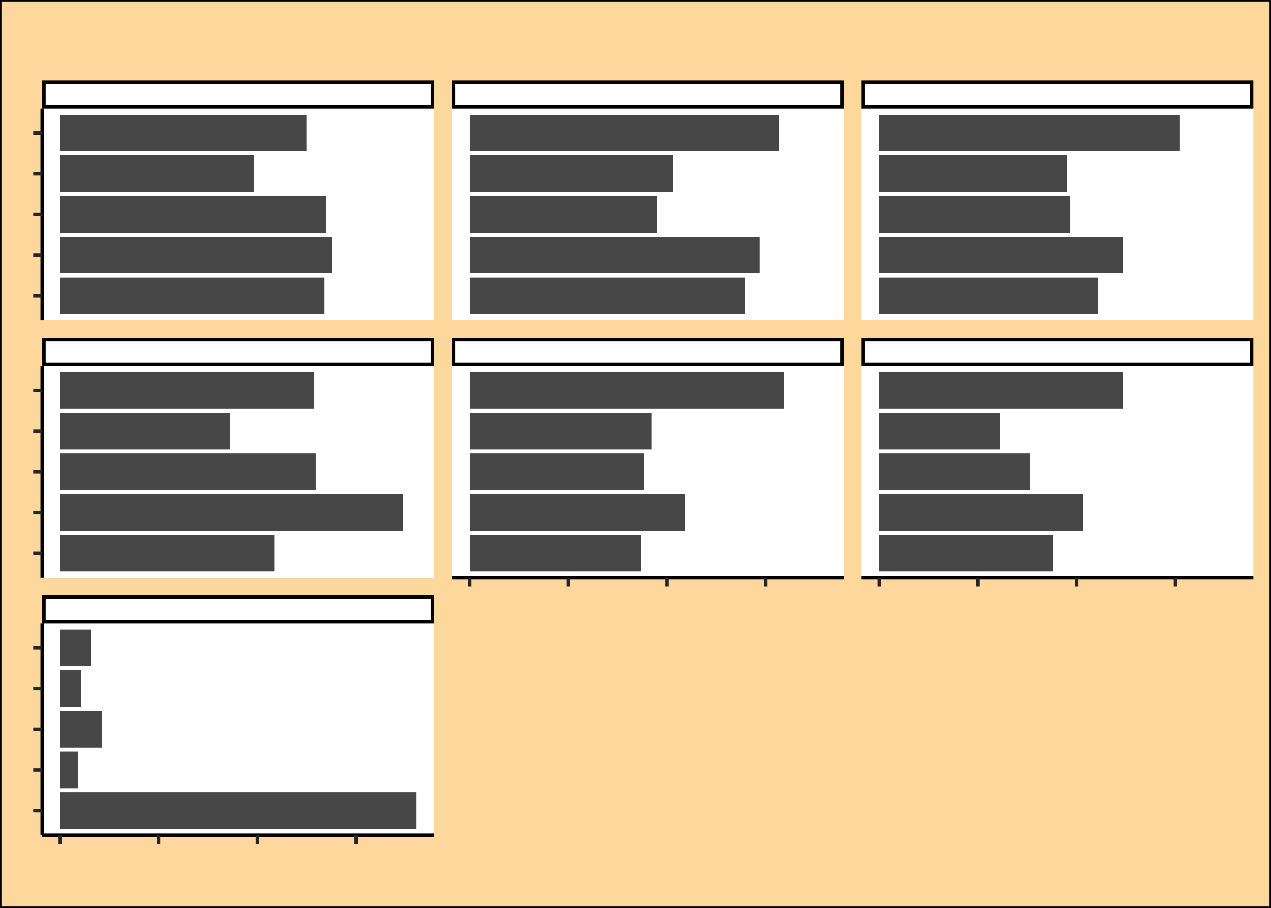
Task and Discussion

Complete the Data Dictionary. Create the graph shown and discuss the following questions:

Identify the type of plot
What are the variables used to plot this graph?
If you were to invest in movie production ventures, which are the two best genres that you might decide to invest in?
Which R command might have been used to obtain the separate plots for each distributor?
If the original dataset had BUDGETS and PROFITS in separate columns, what preprocessing might have been done to achieve this plot?