Setting up R Packages
Plot Theme
Show the Code
# Chunk options
knitr::opts_chunk$set(
  fig.width = 7,
  fig.asp = 0.618, # Golden Ratio
  # out.width = "80%",
  fig.align = "center"
)
##
## https://stackoverflow.com/questions/36476751/associate-a-color-palette-with-ggplot2-theme
##
my_colours <- c("#fd7f6f", "#7eb0d5", "#b2e061", "#bd7ebe", "#ffb55a", "#ffee65", "#beb9db", "#fdcce5", "#8bd3c7")
my_pastels <- c("#66C5CC", "#F6CF71", "#F89C74", "#DCB0F2", "#87C55F", "#9EB9F3", "#FE88B1", "#C9DB74", "#8BE0A4", "#B497E7", "#D3B484", "#B3B3B3")
my_greys <- c("#000000", "#333333", "#666666", "#999999", "#cccccc")
my_vivids <- c("#E58606", "#5D69B1", "#52BCA3", "#99C945", "#CC61B0", "#24796C", "#DAA51B", "#2F8AC4", "#764E9F", "#ED645A", "#CC3A8E", "#A5AA99")

my_bolds <- c("#7F3C8D", "#11A579", "#3969AC", "#F2B701", "#E73F74", "#80BA5A", "#E68310", "#008695", "#CF1C90", "#f97b72", "#4b4b8f", "#A5AA99")

font <- "Roboto Condensed"
mytheme <- theme_classic(base_size = 14) + ### %+replace%    #replace elements we want to change

  theme(
    text = element_text(family = font),
    panel.grid.minor = element_blank(),
    # text elements
    plot.title = element_text(
      family = font,
      face = "bold",
      hjust = 0, # left align
      # vjust = 2 #raise slightly
      margin = margin(0, 0, 10, 0)
    ),
    plot.subtitle = element_text(
      family = font,
      hjust = 0,
      margin = margin(2, 0, 5, 0)
    ),
    plot.caption = element_text(
      family = font,
      size = 8,
      hjust = 1
    ),
    # right align

    axis.title = element_text( # axis titles
      family = font, # font family
      size = 10
    ), # font size
    axis.text = element_text( # axis text
      family = font, # axis family
      size = 8
    ) # font size
  )
theme_av <- list(
  mytheme,
  scale_colour_manual(values = my_bolds, aesthetics = c("colour", "fill"))
)
Introduction
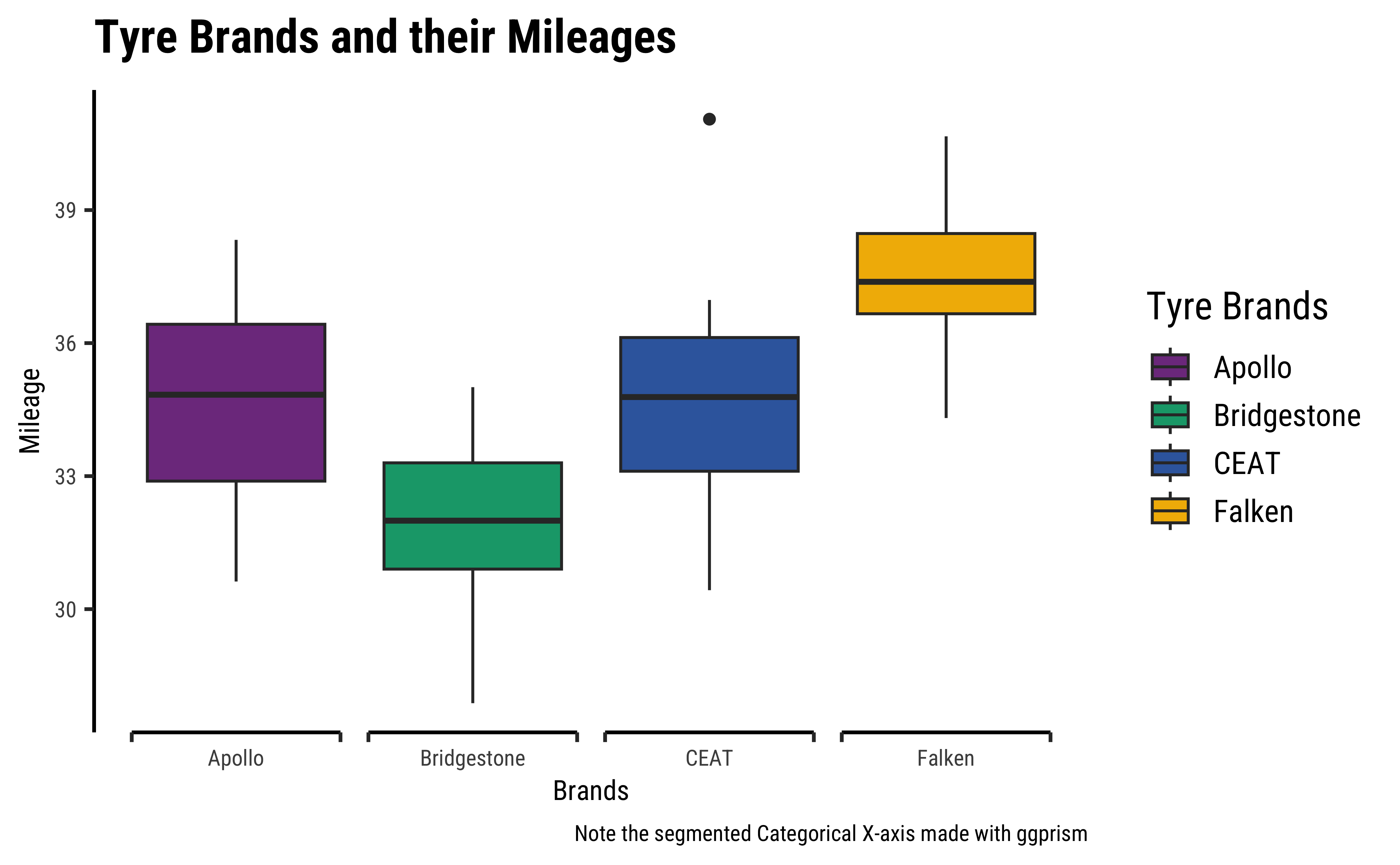
This is a dataset pertaining to tyres from different companies and their lifetime mileages.
Data
Brands <fct> | Mileage <dbl> | |||
|---|---|---|---|---|
| Apollo | 32.99800 | |||
| Apollo | 36.43500 | |||
| Apollo | 32.77700 | |||
| Apollo | 37.63700 | |||
| Apollo | 36.30400 | |||
| Apollo | 35.91500 | |||
| Apollo | 34.70000 | |||
| Apollo | 32.37900 | |||
| Apollo | 33.63100 | |||
| Apollo | 36.41900 |
Download the Modified data
Data Dictionary
Quantitative Variables
Write in.
Qualitative Variables
Write in.
Observations
Write in.
Plot the Data
Task and Discussion: ANOVA
- Complete the pre-analysis steps for ANOVA
Write in.
Model + Table
- Create the ANOVA model
- Create the ANOVA table using the
supernovapackage
Call:
   aov(formula = Mileage ~ Brands, data = tyre)

Terms:
                  Brands Residuals
Sum of Squares  256.2908  266.6495
Deg. of Freedom        3        56

Residual standard error: 2.182108
Estimated effects may be unbalanced
Analysis of Variance Table (Type III SS)
Model: Mileage ~ Brands
SS df MS F PRE p
----- --------------- | ------- -- ------ ------ ----- -----
Model (error reduced) | 256.291 3 85.430 17.942 .4901 .0000
Error (from model) | 266.649 56 4.762
----- --------------- | ------- -- ------ ------ ----- -----
Total (empty model) | 522.940 59 8.863 Post-hoc Analysis and Plots
- Compute the post-hoc differences in means and plot the pair-wise difference plots
  group_1     group_2       diff pooled_se      q    df  lower  upper  p_adj
  <chr>       <chr>        <dbl>     <dbl>  <dbl> <int>  <dbl>  <dbl>  <dbl>
1 Bridgestone Apollo      -3.019     0.563 -5.358    56 -5.129 -0.909  .0021
2 CEAT        Apollo      -0.038     0.563 -0.067    56 -2.148  2.072 1.0000
3 Falken      Apollo       2.826     0.563  5.015    56  0.716  4.935  .0043
4 CEAT        Bridgestone  2.981     0.563  5.291    56  0.871  5.091  .0024
5 Falken      Bridgestone  5.845     0.563 10.373    56  3.735  7.954  .0000
6 Falken      CEAT         2.863     0.563  5.082    56  0.754  4.973  .0037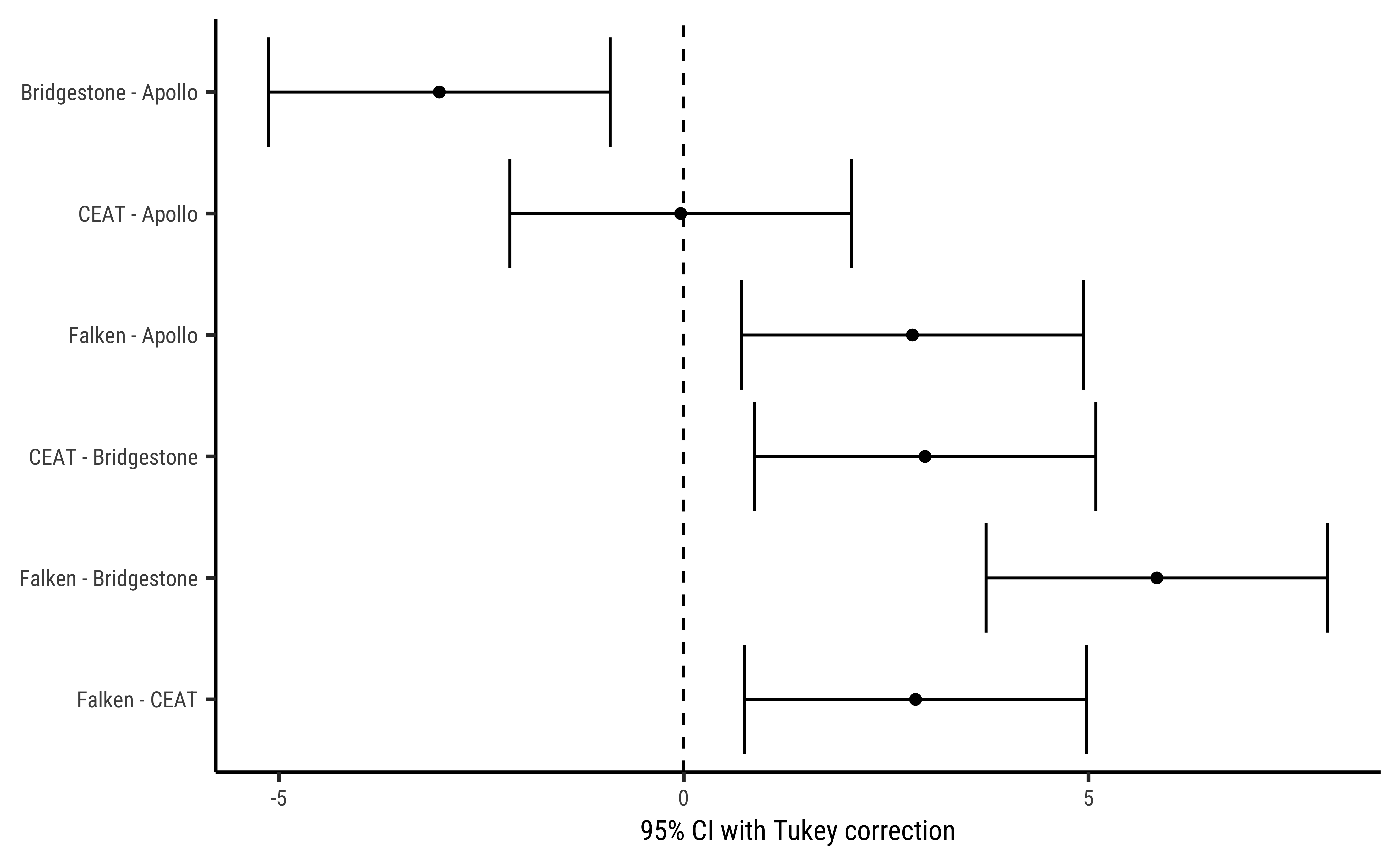
Conclusion
- State a conclusion about the effect of
BrandsonMileage.
Write in.