🃏 Inference for Two Independent Means

How different are you?

To be nobody but myself – in a world which is doing its best, night and day, to make you everybody else – means to fight the hardest battle which any human being can fight, and never stop fighting.

— E.E. Cummings, poet (14 Oct 1894-1962)

Setting up R Packages

library(tidyverse)
library(mosaic) # Our go-to package
library(ggformula)
library(infer) # An alternative package for inference using tidy data
library(broom) # Clean test results in tibble form
library(skimr) # data inspection
library(resampledata3) # Datasets from Chihara and Hesterberg's book
library(openintro) # datasets
library(gt) # for tables
##
library(visStatistics) # All-in-one Stats test package

Plot Theme

# https://stackoverflow.com/questions/74491138/ggplot-custom-fonts-not-working-in-quarto

# Chunk options
knitr::opts_chunk$set(
  fig.width = 7,
  fig.asp = 0.618, # Golden Ratio
  # out.width = "80%",
  fig.align = "center", tidy = "styler",
  tidy.opts = "tidyverse"
)
### Ggplot Theme
### https://rpubs.com/mclaire19/ggplot2-custom-themes

theme_custom <- function() {
  font <- "Roboto Condensed" # assign font family up front

  theme_classic(base_size = 14) %+replace% # replace elements we want to change

    theme(
      panel.grid.minor = element_blank(), # strip minor gridlines
      text = element_text(family = font),
      # text elements
      plot.title = element_text( # title
        family = font, # set font family
        # size = 20,               #set font size
        face = "bold", # bold typeface
        hjust = 0, # left align
        # vjust = 2                #raise slightly
        margin = margin(0, 0, 10, 0)
      ),
      plot.title.position = "plot", # left align title
      plot.subtitle = element_text( # subtitle
        family = font, # font family
        # size = 14,                #font size
        hjust = 0,
        margin = margin(2, 0, 5, 0)
      ),
      plot.subtitle.position = "plot", # left align subtitle

      plot.caption = element_text( # caption
        family = font, # font family
        size = 8, # font size
        hjust = 1
      ), # right align

      axis.title = element_text( # axis titles
        family = font, # font family
        size = 10 # font size
      ),
      plot.caption.position = "plot", # right align caption

      axis.text = element_text( # axis text
        family = font, # axis family
        size = 8
      ) # font size
    )
}

# Set graph theme
theme_set(new = theme_custom())

Introduction

Case Study #1: A Simple Data set with Two Quant Variables

Let us look at the MathAnxiety dataset from the package resampledata. Here we have “anxiety” scores for boys and girls, for different components of mathematics.

Inspecting and Charting Data

data("MathAnxiety", package = "resampledata")
MathAnxiety
MathAnxiety_inspect <- inspect(MathAnxiety)
MathAnxiety_inspect$categorical
MathAnxiety_inspect$quantitative

ABCDEFGHIJ0123456789

Age <dbl>	Gender <fct>	Grade <fct>	AMAS <int>	RCMAS <int>	Arith <int>
137.8	Boy	Secondary	9	20	6
140.7	Boy	Secondary	18	8	6
137.9	Girl	Secondary	23	26	5
142.8	Girl	Secondary	19	18	7
135.6	Boy	Secondary	23	20	1
135.0	Girl	Secondary	27	33	1
133.6	Boy	Secondary	22	23	4
139.3	Boy	Secondary	17	11	7
131.7	Girl	Secondary	28	32	2
134.8	Boy	Secondary	20	30	6

Next

123456

...

60

Previous

1-10 of 599 rows

ABCDEFGHIJ0123456789

name <chr>	class <chr>	levels <int>	n <int>	missing <int>	distribution <chr>
Gender	factor	2	599	0	Boy (53.9%), Girl (46.1%)
Grade	factor	2	599	0	Primary (66.9%), Secondary (33.1%)

2 rows

ABCDEFGHIJ0123456789

	name <chr>	class <chr>	min <dbl>	Q1 <dbl>	median <dbl>	Q3 <dbl>	max <dbl>	mean <dbl>	sd <dbl>
1	Age	numeric	3.7	106.15	120.8	141.85	187.5	124.64925	22.311218
2	AMAS	integer	4.0	18.00	22.0	26.50	45.0	21.98164	6.597962
3	RCMAS	integer	1.0	14.00	19.0	25.00	41.0	19.24040	7.566802
4	Arith	integer	0.0	4.00	6.0	7.00	8.0	5.30217	2.105220

4 rows | 1-10 of 12 columns

We have ~600 data entries, and with 4 Quant variables; Age,AMAS, RCMAS, and AMAS; and two Qual variables, Gender and Grade. A simple dataset, with enough entries to make it worthwhile to explore as our first example.

NoteResearch Question

Is there a difference between boy and girl “anxiety” levels for AMAS (test) in the population from which the MathAnxiety dataset is a sample?

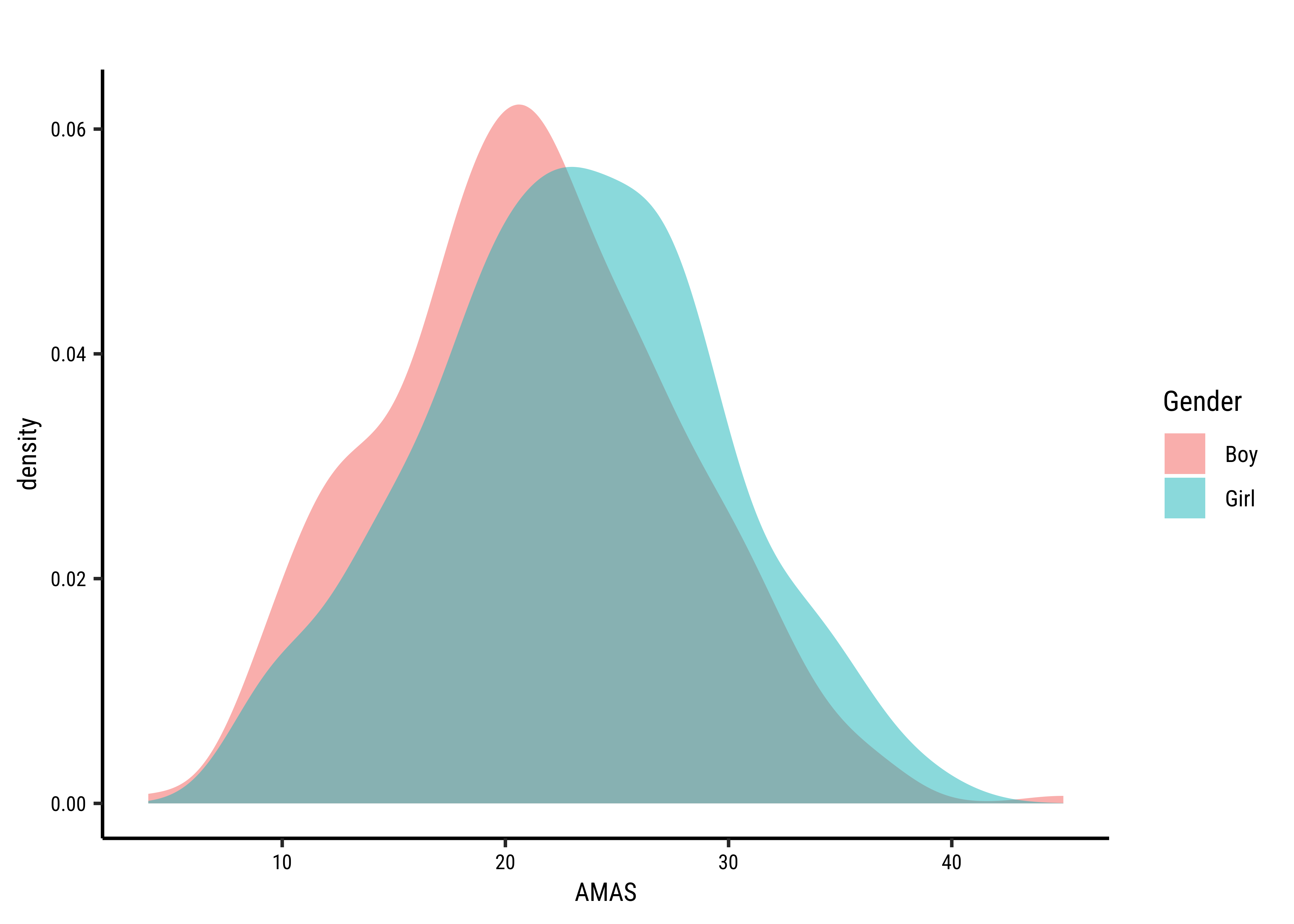
First, histograms, densities and counts of the variable we are interested in, after converting data into long format:

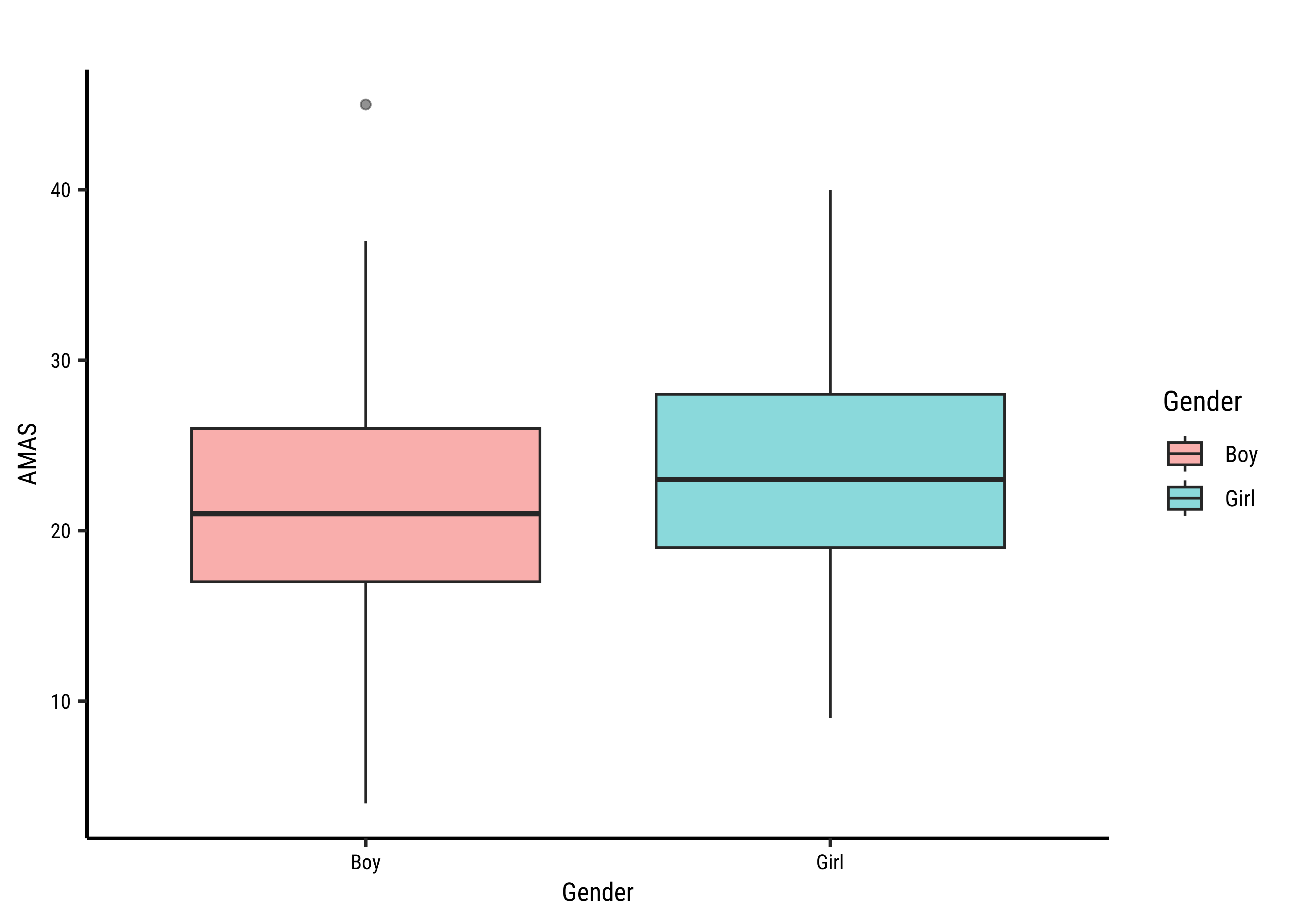
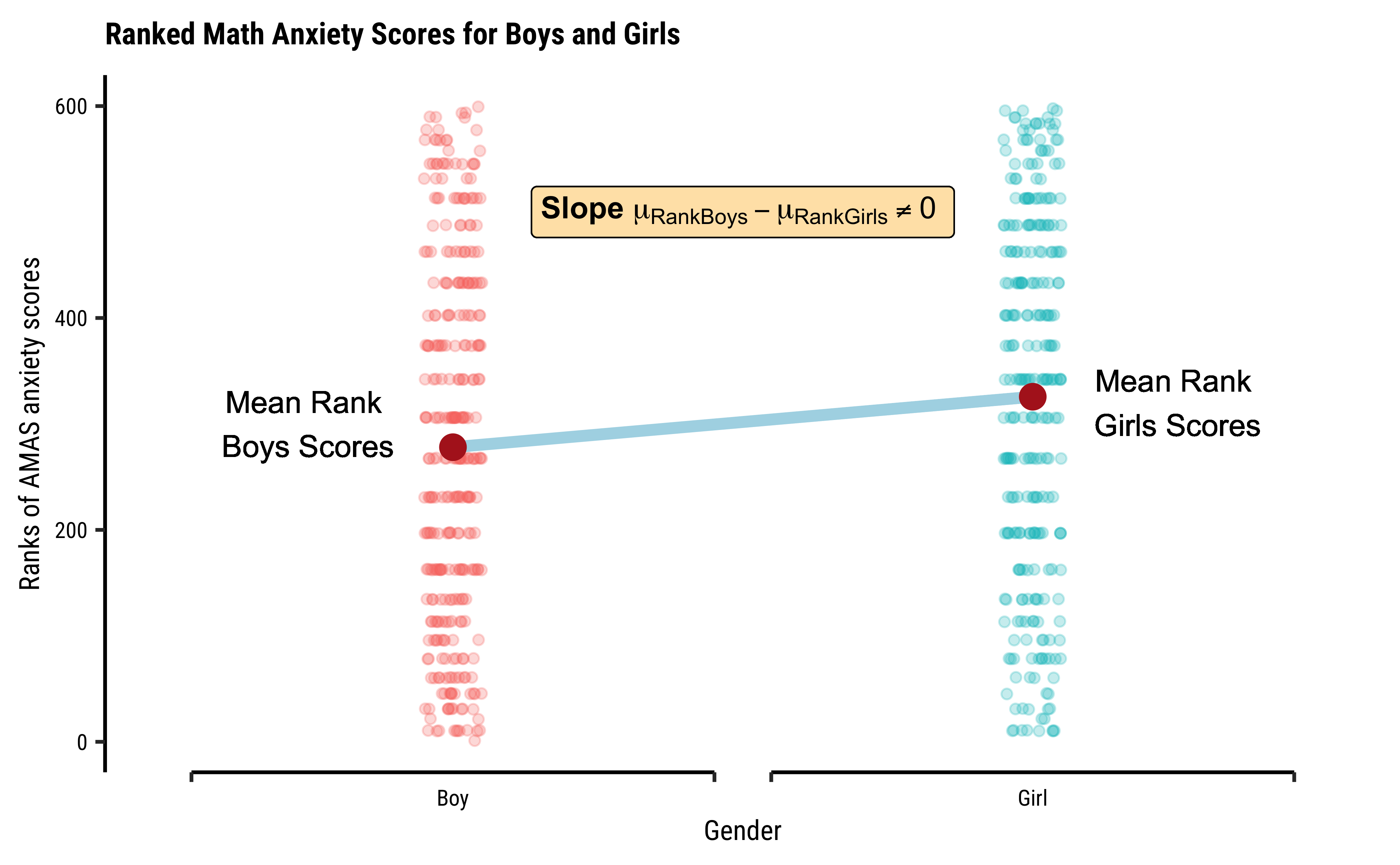
# Set graph theme
theme_set(new = theme_custom())
#
MathAnxiety %>%
  gf_density(
    ~AMAS,
    fill = ~Gender,
    alpha = 0.5,
    title = "Math Anxiety Score Densities",
    subtitle = "Boys vs Girls"
  )
##
MathAnxiety %>%
  pivot_longer(
    cols = -c(Gender, Age, Grade),
    names_to = "type",
    values_to = "value"
  ) %>%
  dplyr::filter(type == "AMAS") %>%
  gf_jitter(
    value ~ Gender,
    group = ~type, color = ~Gender,
    width = 0.08, alpha = 0.3,
    ylab = "AMAS Anxiety Scores",
    title = "Math Anxiety Score Jitter Plots",
    subtitle = "Illustrating Difference in Means"
  ) %>%
  gf_summary(geom = "point", size = 3, colour = "black") %>%
  gf_line(
    stat = "summary", linewidth = 1,
    geom = "line", colour = ~"MeanDifferenceLine"
  )
##
MathAnxiety %>% count(Gender)
MathAnxiety %>%
  group_by(Gender) %>%
  summarise(mean = mean(AMAS))

ABCDEFGHIJ0123456789

Gender <fct>	n <int>
Boy	323
Girl	276

2 rows

ABCDEFGHIJ0123456789

Gender <fct>	mean <dbl>
Boy	21.16718
Girl	22.93478

2 rows

The distributions for anxiety scores for boys and girls overlap considerably and are very similar, though the boxplot for boys shows a significant outlier. Are they close to being normal distributions too? We should check.

A. Check for Normality

Statistical tests for means usually require a couple of checks^{1 2}:

• Are the data normally distributed?
  
• Are the data variances similar?

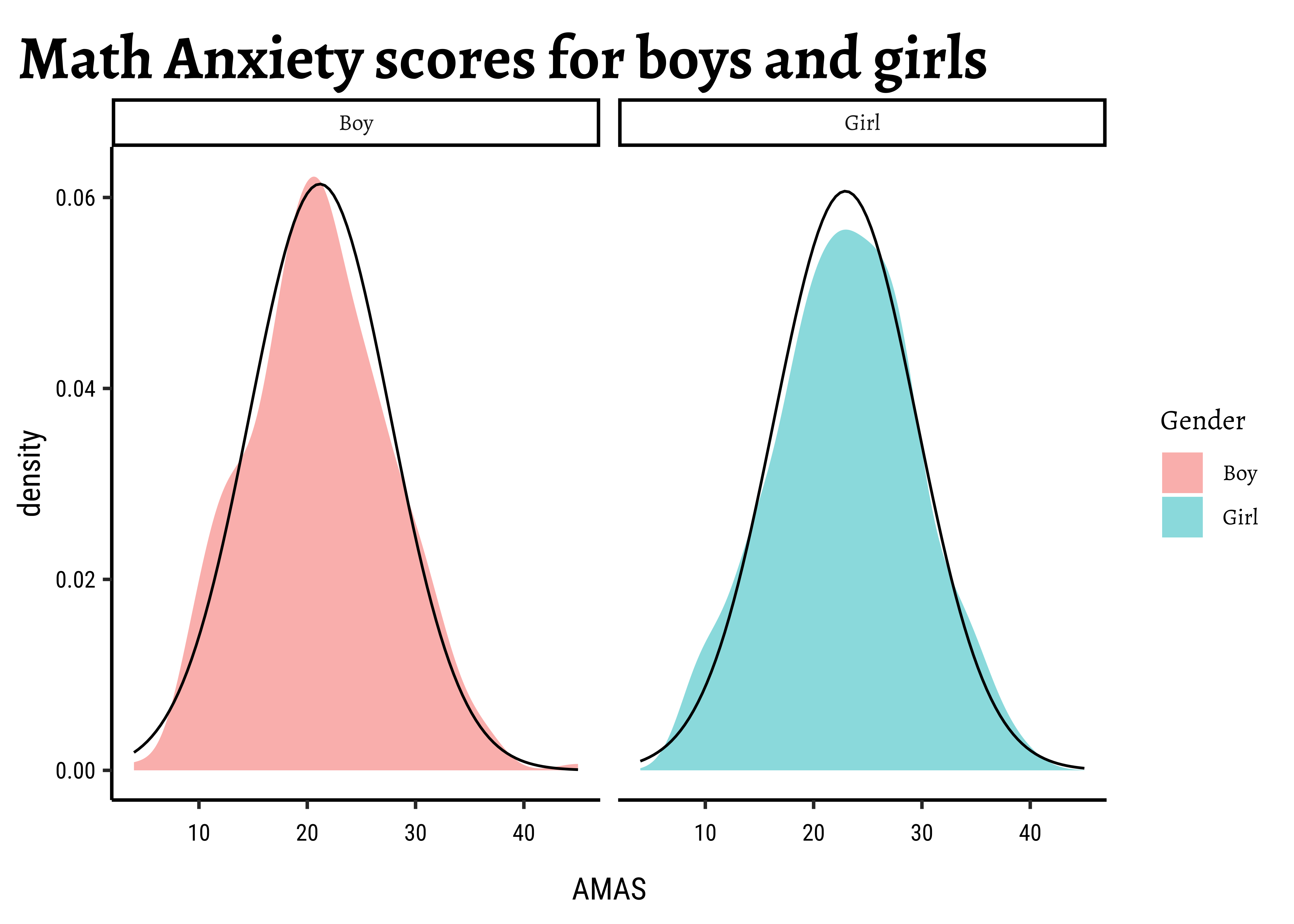
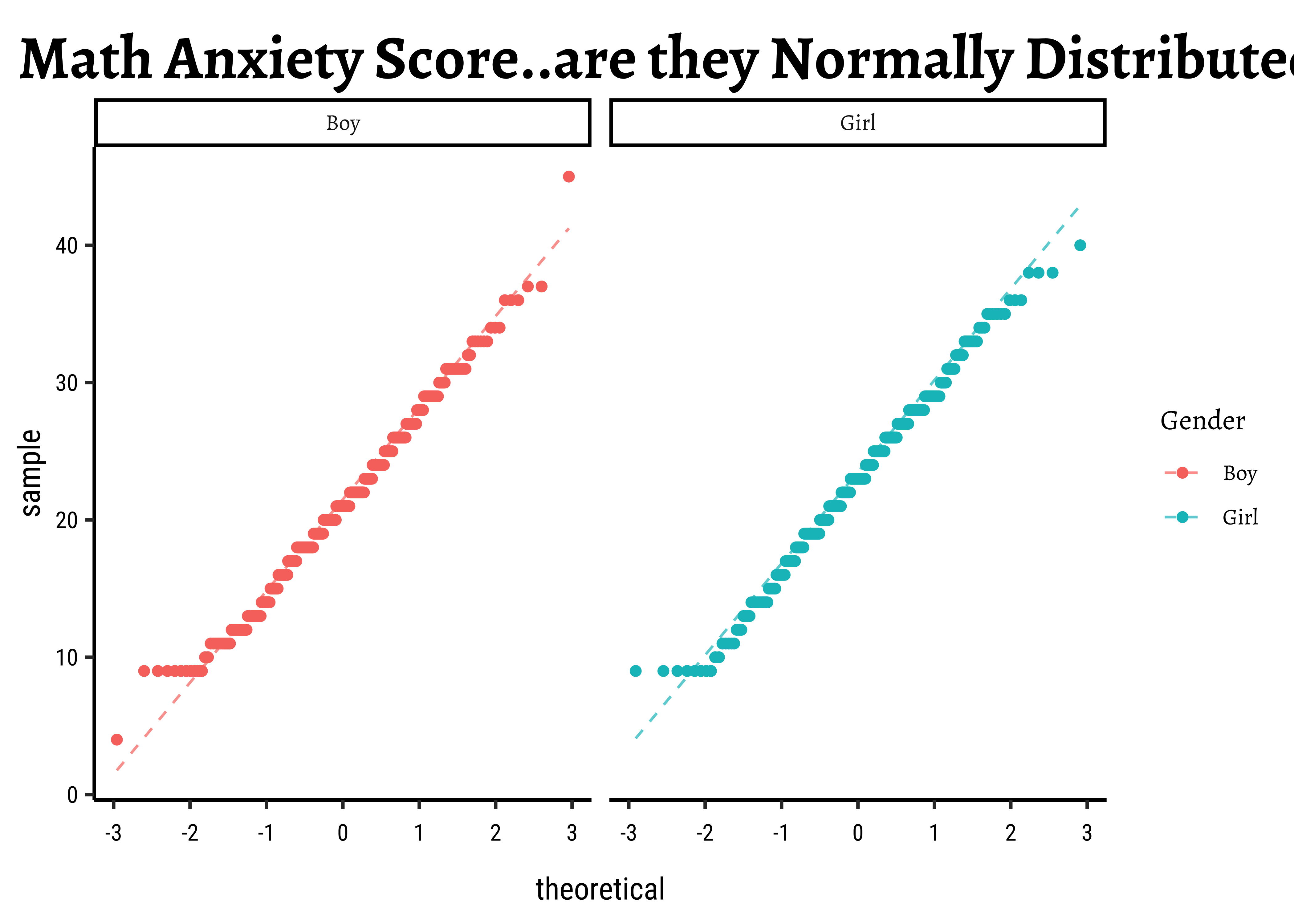
Let us complete a check for normality: the shapiro.wilk test checks whether a Quant variable is from a normal distribution; the NULL hypothesis is that the data are from a normal distribution. We will also look at Q-Q plots for both variables:

# Set graph theme
theme_set(new = theme_custom())
#
MathAnxiety %>%
  gf_density(~AMAS,
    fill = ~Gender,
    alpha = 0.5,
    title = "Math Anxiety scores for boys and girls"
  ) %>%
  gf_facet_grid(~Gender) %>%
  gf_fitdistr(dist = "dnorm")
##
MathAnxiety %>%
  gf_qqline(~AMAS,
    color = ~Gender,
    title = "Math Anxiety Score..are they Normally Distributed?"
  ) %>%
  gf_qq() %>%
  gf_facet_wrap(~Gender) # independent y-axis

Let us split the dataset into subsets, to execute the normality check test (Shapiro-Wilk test):

boys_AMAS <- MathAnxiety %>%
  filter(Gender == "Boy") %>%
  select(AMAS)
##
girls_AMAS <- MathAnxiety %>%
  filter(Gender == "Girl") %>%
  select(AMAS)

shapiro.test(boys_AMAS$AMAS)
shapiro.test(girls_AMAS$AMAS)

    Shapiro-Wilk normality test

data:  boys_AMAS$AMAS
W = 0.99043, p-value = 0.03343

    Shapiro-Wilk normality test

data:  girls_AMAS$AMAS
W = 0.99074, p-value = 0.07835

The distributions for anxiety scores for boys and girls are almost normal, visually speaking. With the Shapiro-Wilk test we find that the scores for girls are normally distributed, but the boys scores are not so. Sigh.

Note

The p.value obtained in the shapiro.wilk test suggests the chances of the data being so, given the Assumption that they are normally distributed.

We see that MathAnxiety contains discrete-level scores for anxiety for the two variables (for Boys and Girls) anxiety scores. The boys score has a significant outlier, which we saw earlier and perhaps that makes that variable lose out, perhaps narrowly.

B. Check for Variances

Let us check if the two variables have similar variances: the var.test does this for us, with a NULL hypothesis that the variances are not significantly different:

var.test(AMAS ~ Gender,
  data = MathAnxiety,
  conf.int = TRUE, conf.level = 0.95
) %>%
  broom::tidy()

ABCDEFGHIJ0123456789

estimate <dbl>	num.df <int>	den.df <int>	statistic <dbl>	p.value <dbl>	conf.low <dbl>	conf.high <dbl>	method <chr>
0.9752474	322	275	0.9752474	0.8268198	0.7755891	1.223763	F test to compare two variances

1 row | 1-8 of 9 columns

##
qf(0.975, 275, 322)

[1] 1.254823

The variances are quite similar as seen by the $p.value=0.82$. We also saw it visually when we plotted the overlapped distributions earlier.

ImportantConditions:

1. The two variables are not both normally distributed.
2. The two variances are significantly similar.

Hypothesis

Based on the graphs, how would we formulate our Hypothesis? We wish to infer whether there is any difference in the mean anxiety score between Girls and Boys, in the population from which the dataset MathAnxiety has been drawn. So accordingly:

$$H_0:{\mu }_{Boys}={\mu }_{Girls}$$

$$H_a:{\mu }_{Girls}\ne {\mu }_{Boys}$$

Observed and Test Statistic

What would be the test statistic we would use? The difference in means. Is the observed difference in the means between the two groups of scores non-zero? We use the diffmean function:

obs_diff_amas <- diffmean(AMAS ~ Gender, data = MathAnxiety)
obs_diff_amas

diffmean 
  1.7676 

Girls’ AMAS anxiety scores are, on average, $1.76$ points higher than those for Boys in the dataset/sample.

NoteOn Observed Difference Estimates

Different tests here will show the difference as positive or negative, but with the same value! This depends upon the way the factor variable Gender is used, i.e. Boy-Girl or Girl-Boy…

Inference

Using the Parametric t.test

Since the data are not both normally distributed, though the variances similar, we typically cannot use a parametric t.test. However, we can still examine the results:

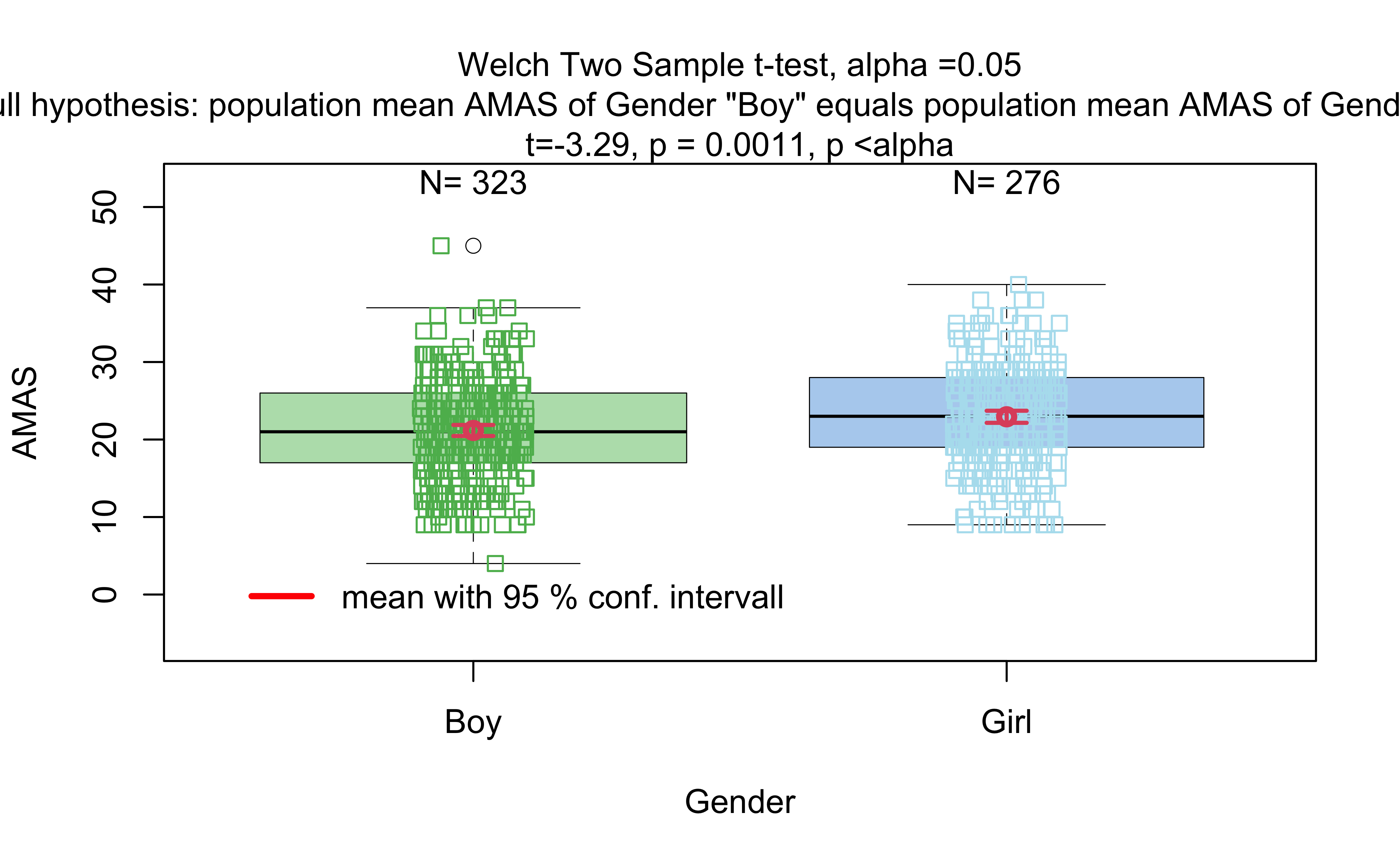
mosaic::t_test(AMAS ~ Gender, data = MathAnxiety) %>%
  broom::tidy()

ABCDEFGHIJ0123456789

estimate <dbl>	estimate1 <dbl>	estimate2 <dbl>	statistic <dbl>	p.value <dbl>	parameter <dbl>	conf.low <dbl>	conf.high <dbl>
-1.7676	21.16718	22.93478	-3.291843	0.001055808	580.2004	-2.822229	-0.7129706

1 row | 1-8 of 10 columns

The p.value is $0.001$ ! And the Confidence Interval does not straddle $0$. So the t.test gives us good reason to reject the Null Hypothesis that the means are similar and that there is a significant difference between Boys and Girls when it comes to AMAS anxiety. But can we really believe this, given the non-normality of data?

Using the Mann-Whitney Test

Since the data variables do not satisfy the assumption of being normally distributed, and though the variances are similar, we use the classical wilcox.test (Type help(wilcox.test) in your Console.) which implements what we need here: the Mann-Whitney U test:³

The Mann-Whitney test as a test of mean ranks. It first ranks all your values from high to low, computes the mean rank in each group, and then computes the probability that random shuffling of those values between two groups would end up with the mean ranks as far apart as, or further apart, than you observed. No assumptions about distributions are needed so far. (emphasis mine)

$$mean(rank(AMA{S}_{Girls}))-mean(rank(AMA{S}_{Boys}))=diff$$

$$H_0:{\mu }_{Boys}-{\mu }_{Girls}=0$$

$$H_a:{\mu }_{Boys}-{\mu }_{Girls}\ne 0$$

wilcox.test(AMAS ~ Gender,
  data = MathAnxiety,
  conf.int = TRUE,
  conf.level = 0.95
) %>%
  broom::tidy()

ABCDEFGHIJ0123456789

estimate <dbl>	statistic <dbl>	p.value <dbl>	conf.low <dbl>	conf.high <dbl>
-1.999998	37483	0.0007736219	-2.999947	-0.9999882

1 row | 1-5 of 7 columns

The p.value is very similar, $0.00077$, and again the Confidence Interval does not straddle $0$, and we are hence able to reject the NULL hypothesis that the means are equal and accept the alternative hypothesis that there is a significant difference in mean anxiety scores between Boys and Girls.

Using the Linear Model Interpretation

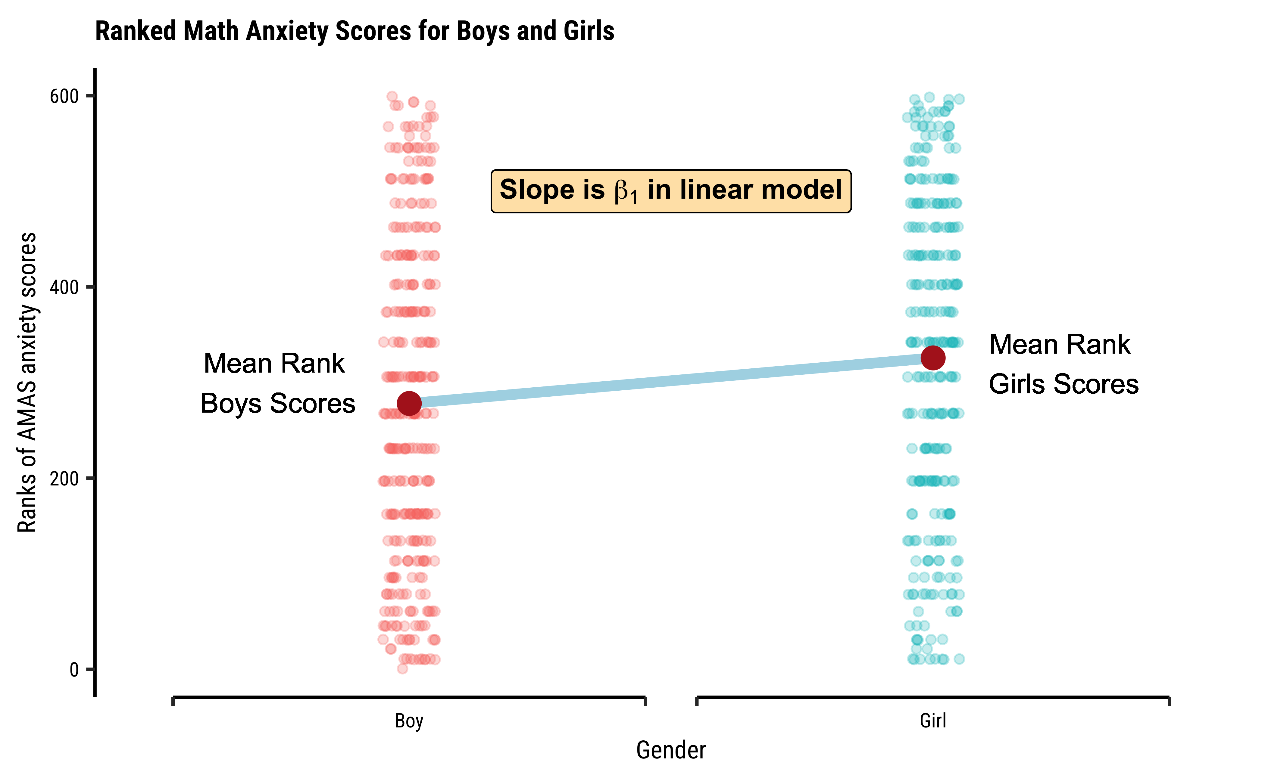
We can apply the linear-model-as-inference interpretation to the ranked data data to implement the non-parametric test as a Linear Model:

$$lm(rank(AMAS)\sim gender)={\beta }_0+{\beta }_1\ast gender$$

$$H_0:{\beta }_1=0$$

$$H_a:{\beta }_1\ne 0$$

lm(rank(AMAS) ~ Gender,
  data = MathAnxiety
) %>%
  broom::tidy(
    conf.int = TRUE,
    conf.level = 0.95
  )

ABCDEFGHIJ0123456789

term <chr>	estimate <dbl>	std.error <dbl>	statistic <dbl>	p.value <dbl>
(Intercept)	278.04644	9.535561	29.158898	6.848992e-117
GenderGirl	47.64559	14.047696	3.391701	7.405210e-04

2 rows | 1-5 of 7 columns

TipDummy Variables in lm

Note how the Qual variable was used here in Linear Regression! The Gender variable was treated as a binary “dummy” variable⁴.

Here too we see that the p.value for the slope term (“GenderGirl”) is significant at $7.4\ast {10}^{-4}$.

Using the Permutation Test

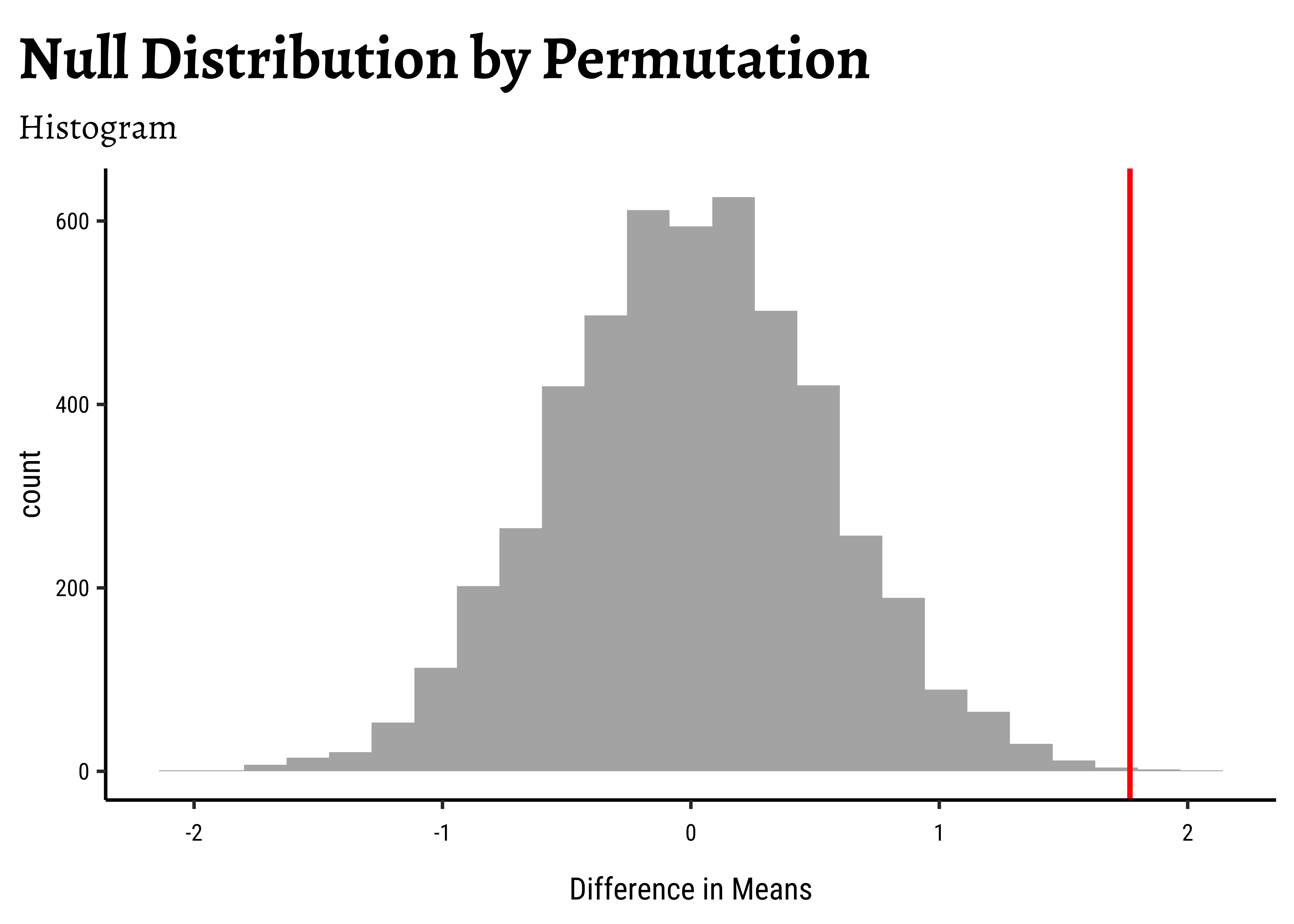
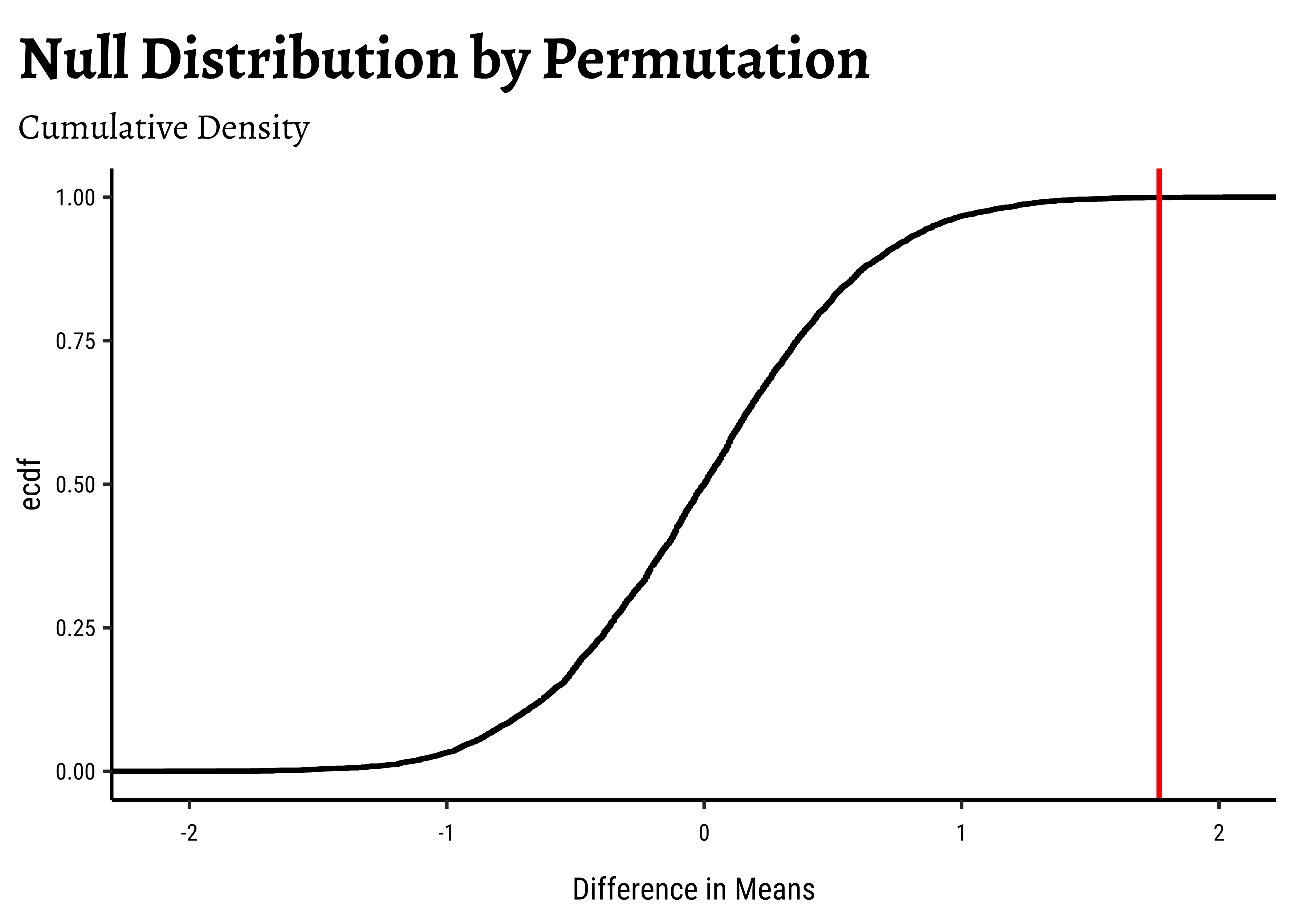
We pretend that Gender has no effect on the AMAS anxiety scores. If this is our position, then the Gender labels are essentially meaningless, and we can pretend that any AMAS score belongs to a Boy or a Girl. This means we can mosaic::shuffle (permute) the Gender labels and see how uncommon our real data is. And we do not have to really worry about whether the data are normally distributed, or if their variances are nearly equal.

Important

The “pretend” position is exactly the NULL Hypothesis!! The “uncommon” part is the p.value under NULL!!

null_dist_amas <-
  do(4999) * diffmean(data = MathAnxiety, AMAS ~ shuffle(Gender))
null_dist_amas

ABCDEFGHIJ0123456789

diffmean <dbl>
-0.1742383452
0.3229797640
-0.7050522726
0.2154731458
-0.4430048907
0.9411428187
-0.8663121999
-0.0196975815
0.7530062368
-0.0600125634

Next

123456

...

500

Previous

1-10 of 4,999 rows

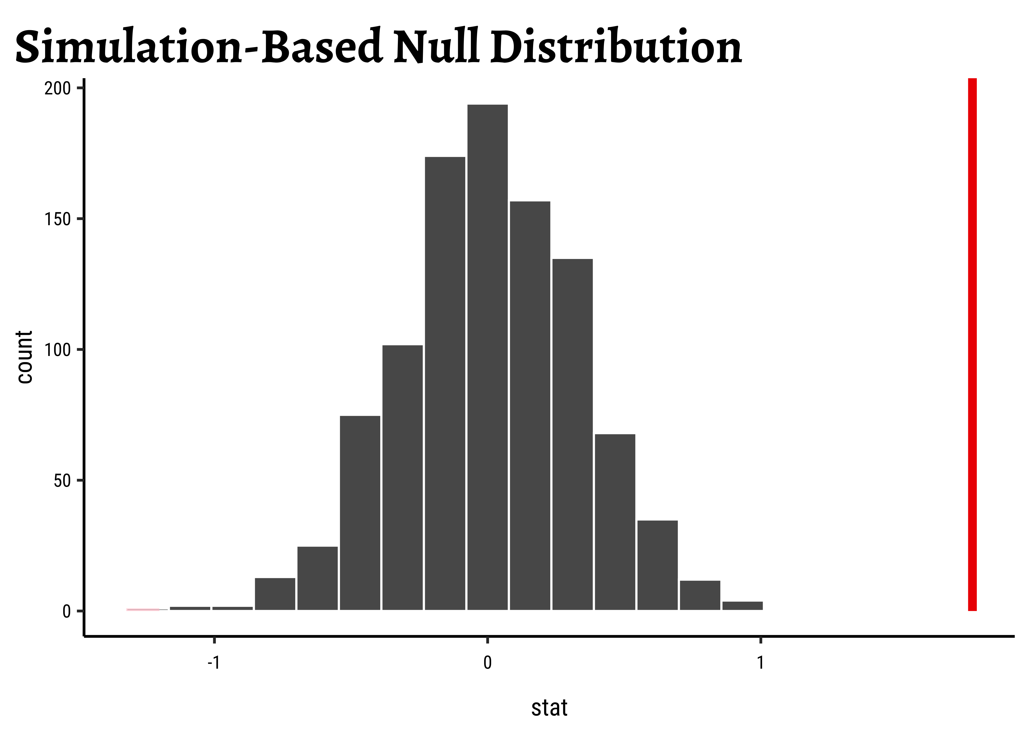
# Set graph theme
theme_set(new = theme_custom())
#
gf_histogram(data = null_dist_amas, ~diffmean, bins = 25) %>%
  gf_vline(
    xintercept = obs_diff_amas,
    colour = "red", linewidth = 1,
    title = "Null Distribution by Permutation",
    subtitle = "Histogram"
  ) %>%
  gf_labs(x = "Difference in Means")
###
gf_ecdf(
  data = null_dist_amas, ~diffmean,
  linewidth = 1
) %>%
  gf_vline(
    xintercept = obs_diff_amas,
    colour = "red", linewidth = 1,
    title = "Null Distribution by Permutation",
    subtitle = "Cumulative Density"
  ) %>%
  gf_labs(x = "Difference in Means")

1 - prop1(~ diffmean <= obs_diff_amas, data = null_dist_amas)

prop_TRUE 
    6e-04 

Clearly the observed_diff_amas is much beyond anything we can generate with permutations with gender! And hence there is a significant difference in weights across gender!

All Tests Together

We can put all the test results together to get a few more insights about the tests:

mosaic::t_test(AMAS ~ Gender,
  data = MathAnxiety
) %>%
  broom::tidy() %>%
  gt() %>%
  tab_style(
    style = list(cell_fill(color = "cyan"), cell_text(weight = "bold")),
    locations = cells_body(columns = p.value)
  ) %>%
  tab_header(title = "t.test") %>%
  tab_options(table.font.size = 10)

wilcox.test(AMAS ~ Gender,
  data = MathAnxiety
) %>%
  broom::tidy() %>%
  gt() %>%
  tab_style(
    style = list(cell_fill(color = "cyan"), cell_text(weight = "bold")),
    locations = cells_body(columns = p.value)
  ) %>%
  tab_header(title = "wilcox.test") %>%
  tab_options(table.font.size = 10)

lm(AMAS ~ Gender,
  data = MathAnxiety
) %>%
  broom::tidy(
    conf.int = TRUE,
    conf.level = 0.95
  ) %>%
  gt() %>%
  tab_style(
    style = list(cell_fill(color = "cyan"), cell_text(weight = "bold")),
    locations = cells_body(columns = p.value)
  ) %>%
  tab_header(title = "Linear Model with Original Data") %>%
  tab_options(table.font.size = 10)

lm(rank(AMAS) ~ Gender,
  data = MathAnxiety
) %>%
  broom::tidy(
    conf.int = TRUE,
    conf.level = 0.95
  ) %>%
  gt() %>%
  tab_style(
    style = list(cell_fill(color = "cyan"), cell_text(weight = "bold")),
    locations = cells_body(columns = p.value)
  ) %>%
  tab_header(title = "Linear Model with Ranked Data") %>%
  tab_options(table.font.size = 10)

t.test
estimate	estimate1	estimate2	statistic	p.value	parameter	conf.low	conf.high	method	alternative
-1.7676	21.16718	22.93478	-3.291843	0.001055808	580.2004	-2.822229	-0.7129706	Welch Two Sample t-test	two.sided

wilcox.test
statistic	p.value	method	alternative
37483	0.0007736219	Wilcoxon rank sum test with continuity correction	two.sided

Linear Model with Original Data
term	estimate	std.error	statistic	p.value	conf.low	conf.high
(Intercept)	21.16718	0.3641315	58.130602	5.459145e-248	20.4520482	21.882317
GenderGirl	1.76760	0.5364350	3.295087	1.042201e-03	0.7140708	2.821129

Linear Model with Ranked Data
term	estimate	std.error	statistic	p.value	conf.low	conf.high
(Intercept)	278.04644	9.535561	29.158898	6.848992e-117	259.31912	296.7738
GenderGirl	47.64559	14.047696	3.391701	7.405210e-04	20.05668	75.2345

As we can see, all tests are in agreement that there is a significant effect of Gender on the AMAS anxiety scores!

One Test to Rule Them All: visStatistics

We can use the visStatistics package to run all the tests in one go, using the in-built decision tree. This is a very useful package for teaching statistics, and it can be used to run all the tests we have seen so far, and more. Here goes: we use the visstat function to run all the tests, and then we can summarize the results. The visstat function takes a dataset, a quantitative variable, a qualitative variable, and some options for the tests to run.

From the visStatistics package documentation:

visStatistics automatically selects and visualises appropriate statistical hypothesis tests between two column vectors of type of class “numeric”, “integer”, or “factor”. The choice of test depends on the class, distribution, and sample size of the vectors, as well as the user-defined ‘conf.level’. The main function visstat() visualises the selected test with appropriate graphs (box plots, bar charts, regression lines with confidence bands, mosaic plots, residual plots, Q-Q plots), annotated with the main test results, including any assumption checks and post-hoc analyses.

# Generate the annotated plots and statistics
visstat(
  x = MathAnxiety$Gender,
  y = MathAnxiety$AMAS,
  conf.level = 0.95, numbers = TRUE
) %>%
  summary()

Summary of visstat object

--- Named components ---
[1] "dependent variable (response)"    "independent variables (features)"
[3] "t-test-statistics"                "Shapiro-Wilk-test_sample1"       
[5] "Shapiro-Wilk-test_sample2"       

--- Contents ---

$dependent variable (response):
[1] "AMAS"

$independent variables (features):
[1] Boy  Girl
Levels: Boy Girl

$t-test-statistics:

    Welch Two Sample t-test

data:  x1 and x2
t = -3.2918, df = 580.2, p-value = 0.001056
alternative hypothesis: true difference in means is not equal to 0
95 percent confidence interval:
 -2.8222293 -0.7129706
sample estimates:
mean of x mean of y 
 21.16718  22.93478 


$Shapiro-Wilk-test_sample1:

    Shapiro-Wilk normality test

data:  x
W = 0.99043, p-value = 0.03343


$Shapiro-Wilk-test_sample2:

    Shapiro-Wilk normality test

data:  x
W = 0.99074, p-value = 0.07835


--- Attributes ---
$plot_paths
character(0)

The tool runs the Welch t-test and declares the p-value to be significant. The Shapiro-Wilk test results here also confirm what we had performed earlier. Hence we can say that we may reject the NULL Hypothesis and state that there is a statistically significant difference in AMAS anxiety scores between Boys and Girls.

Case Study #2: Youth Risk Behavior Surveillance System (YRBSS) survey

Every two years, the Centers for Disease Control and Prevention in the USA conduct the Youth Risk Behavior Surveillance System (YRBSS) survey, where it takes data from highschoolers (9th through 12th grade), to analyze health patterns. We will work with a selected group of variables from a random sample of observations during one of the years the YRBSS was conducted.The yrbss dataset is part of the openintro package. Type this in your console: help(yrbss).

Inspecting and Charting Data

data(yrbss, package = "openintro")
yrbss
yrbss_inspect <- inspect(yrbss)
yrbss_inspect$categorical
yrbss_inspect$quantitative

ABCDEFGHIJ0123456789

age <int>	gender <chr>	grade <chr>	hispanic <chr>	race <chr>	height <dbl>	weight <dbl>	helmet_12m <chr>	text_while_driving_30d <chr>
14	female	9	not	Black or African American	NA	NA	never	0
14	female	9	not	Black or African American	NA	NA	never	NA
15	female	9	hispanic	Native Hawaiian or Other Pacific Islander	1.73	84.37	never	30
15	female	9	not	Black or African American	1.60	55.79	never	0
15	female	9	not	Black or African American	1.50	46.72	did not ride	did not drive
15	female	9	not	Black or African American	1.57	67.13	did not ride	did not drive
15	female	9	not	Black or African American	1.65	131.54	did not ride	NA
14	male	9	not	Black or African American	1.88	71.22	never	NA
15	male	9	not	Black or African American	1.75	63.50	never	NA
15	male	10	not	Black or African American	1.37	97.07	did not ride	NA

Next

123456

...

1000

Previous

1-10 of 10,000 rows | 1-9 of 13 columns

ABCDEFGHIJ0123456789

name <chr>	class <chr>	levels <int>	n <int>	missing <int>	distribution <chr>
gender	character	2	13571	12	male (51.2%), female (48.8%)
grade	character	5	13504	79	9 (26.6%), 12 (26.3%), 11 (23.6%) ...
hispanic	character	2	13352	231	not (74.4%), hispanic (25.6%)
race	character	5	10778	2805	White (59.5%) ...
helmet_12m	character	6	13272	311	never (52.6%), did not ride (34.3%) ...
text_while_driving_30d	character	8	12665	918	0 (37.8%), did not drive (36.7%) ...
hours_tv_per_school_day	character	7	13245	338	2 (20.4%), <1 (16.4%), 3 (16.1%) ...
school_night_hours_sleep	character	7	12335	1248	7 (28.1%), 8 (21.8%), 6 (21.5%) ...

8 rows

ABCDEFGHIJ0123456789

	name <chr>	class <chr>	min <dbl>	Q1 <dbl>	median <dbl>	Q3 <dbl>	max <dbl>	mean <dbl>	sd <dbl>
1	age	integer	12.00	15.00	16.00	17.00	18.00	16.157041	1.2637373
2	height	numeric	1.27	1.60	1.68	1.78	2.11	1.691241	0.1046973
3	weight	numeric	29.94	56.25	64.41	76.20	180.99	67.906503	16.8982128
4	physically_active_7d	integer	0.00	2.00	4.00	7.00	7.00	3.903005	2.5641046
5	strength_training_7d	integer	0.00	0.00	3.00	5.00	7.00	2.949948	2.5768522

5 rows | 1-10 of 12 columns

We have 13K data entries, and with 13 different variables, some Qual and some Quant. Many entries are missing too, typical of real-world data and something we will have to account for in our computations. The meaning of each variable can be found by bringing up the help file.

Type this in your console: help(yrbss)

First, histograms, densities and counts of the variable we are interested in:

yrbss_select_gender <- yrbss %>%
  select(weight, gender) %>%
  mutate(gender = as_factor(gender)) %>%
  drop_na(weight) # Sadly dropping off NA data

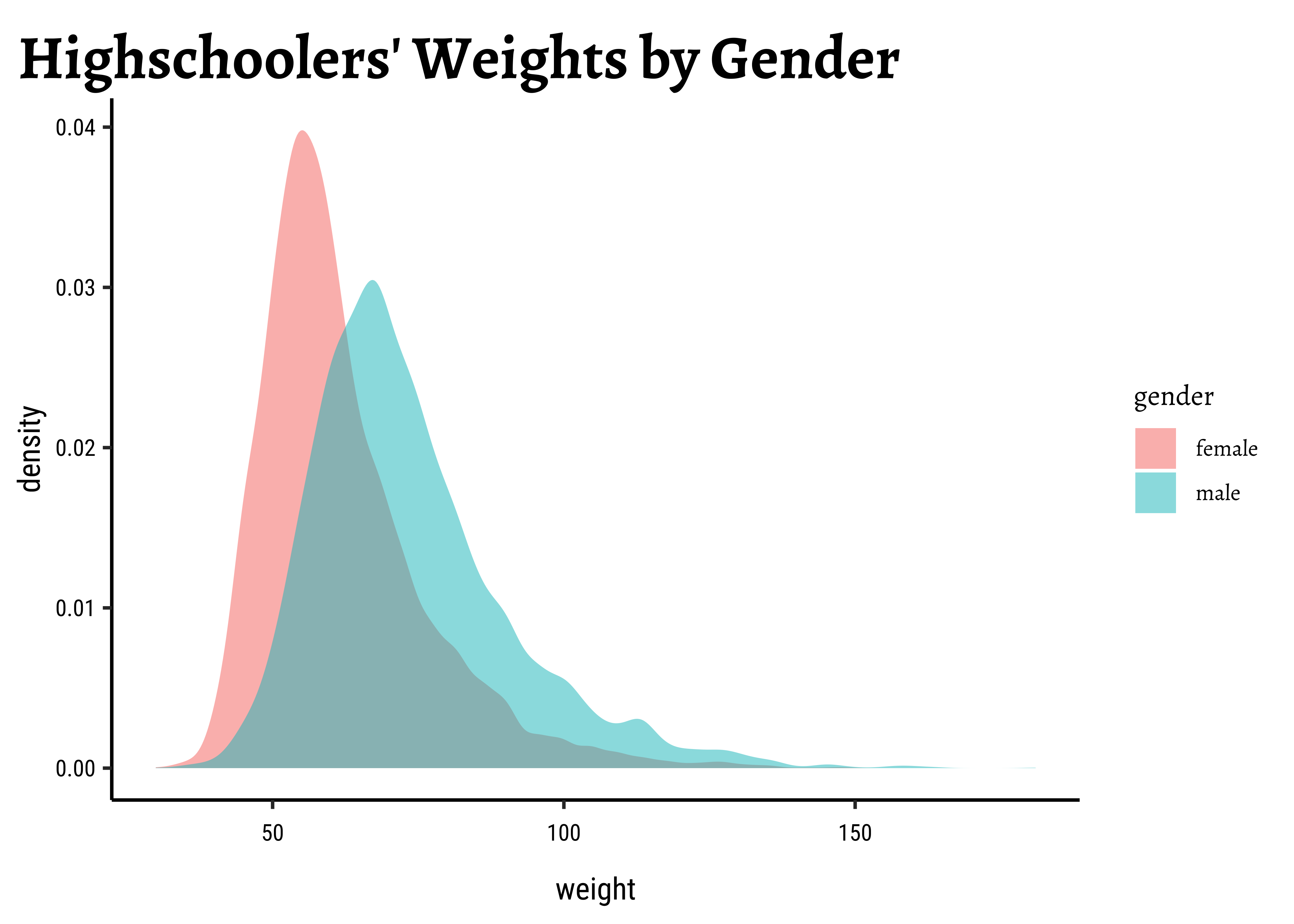
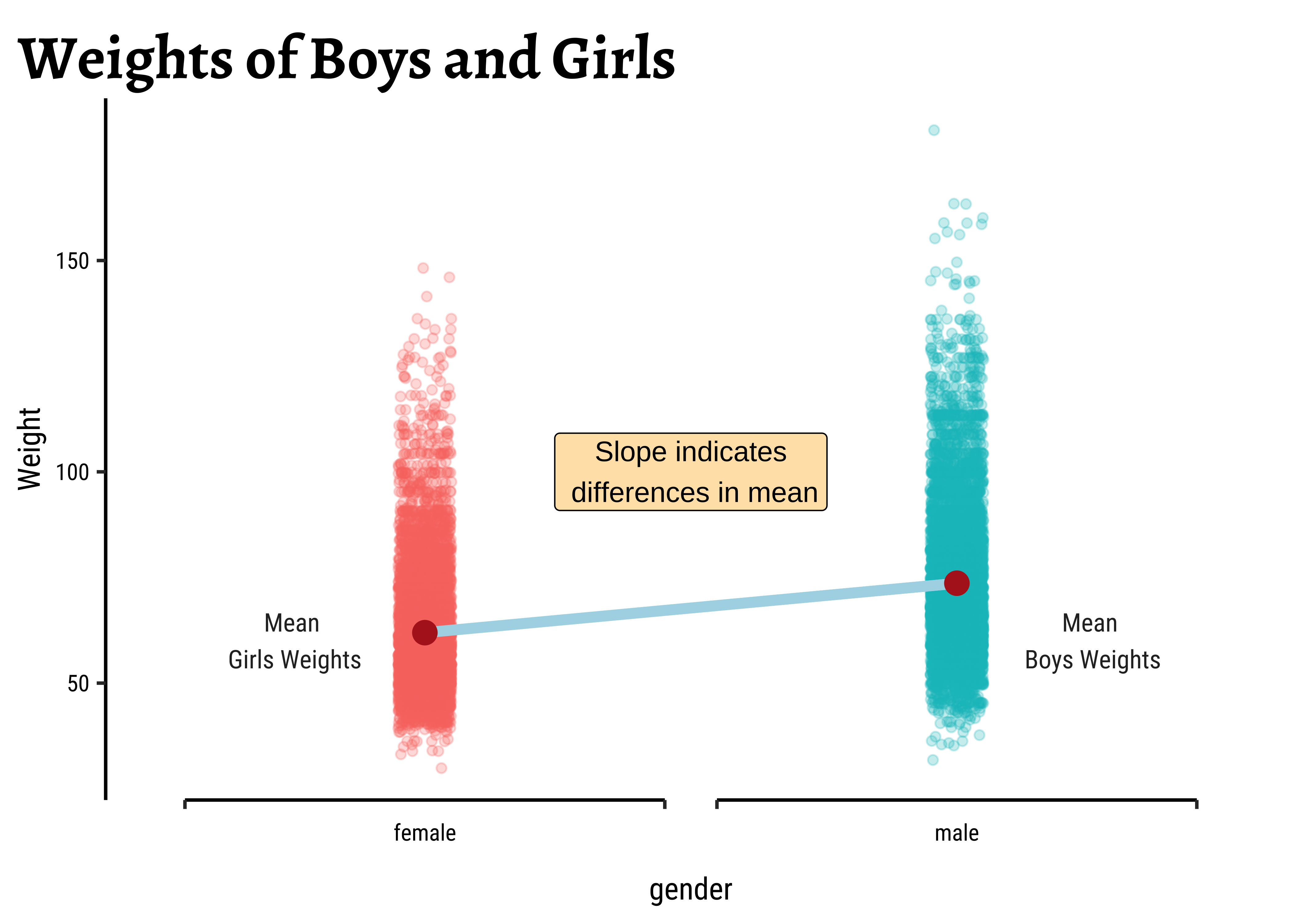
# Set graph theme
theme_set(new = theme_custom())
##
yrbss_select_gender %>%
  gf_density(~weight,
    fill = ~gender,
    alpha = 0.5,
    title = "Highschoolers' Weights by Gender"
  )
###
yrbss_select_gender %>%
  gf_jitter(weight ~ gender,
    color = ~gender,
    show.legend = FALSE,
    width = 0.05, alpha = 0.25,
    ylab = "Weight",
    title = "Weights of Boys and Girls"
  ) %>%
  gf_summary(
    group = ~1, # See the reference link above. Damn!!!
    fun = "mean", geom = "line", colour = "lightblue",
    lty = 1, linewidth = 2
  ) %>%
  gf_summary(
    fun = "mean", colour = "firebrick",
    size = 4, geom = "point"
  ) %>%
  gf_refine(scale_x_discrete(
    breaks = c("male", "female"),
    labels = c("male", "female"),
    guide = "prism_bracket"
  )) %>%
  gf_refine(
    annotate(x = 0.75, y = 60, geom = "text", label = "Mean\n Girls Weights"),
    annotate(x = 2.25, y = 60, geom = "text", label = "Mean\n Boys Weights"),
    annotate(x = 1.5, y = 100, geom = "label", label = "Slope indicates\n differences in mean", fill = "moccasin")
  )

yrbss_select_gender %>% count(gender)

ABCDEFGHIJ0123456789

gender <fct>	n <int>
female	6165
male	6414

2 rows

Overlapped Distribution plot shows some difference in the means; and the Boxplots show visible difference in the medians. In this Case Study, our research question is:

Hypothesis

NoteResearch Question

Does weight of highschoolers in this dataset vary with gender?

Based on the graphs, how would we formulate our Hypothesis? We wish to infer whether there is difference in mean weight across gender. So accordingly:

$$H_0:{\mu }_{weight-male}={\mu }_{weight-female}$$

$$H_a:{\mu }_{weight-male}\ne {\mu }_{weight-female}$$

A. Check for Normality

As stated before, statistical tests for means usually require a couple of checks:

• Are the data normally distributed?
  
• Are the data variances similar?

We will complete a visual check for normality with plots, and since we cannot do a shapiro.test (length(data) >= 5000) we can use the Anderson-Darling test.

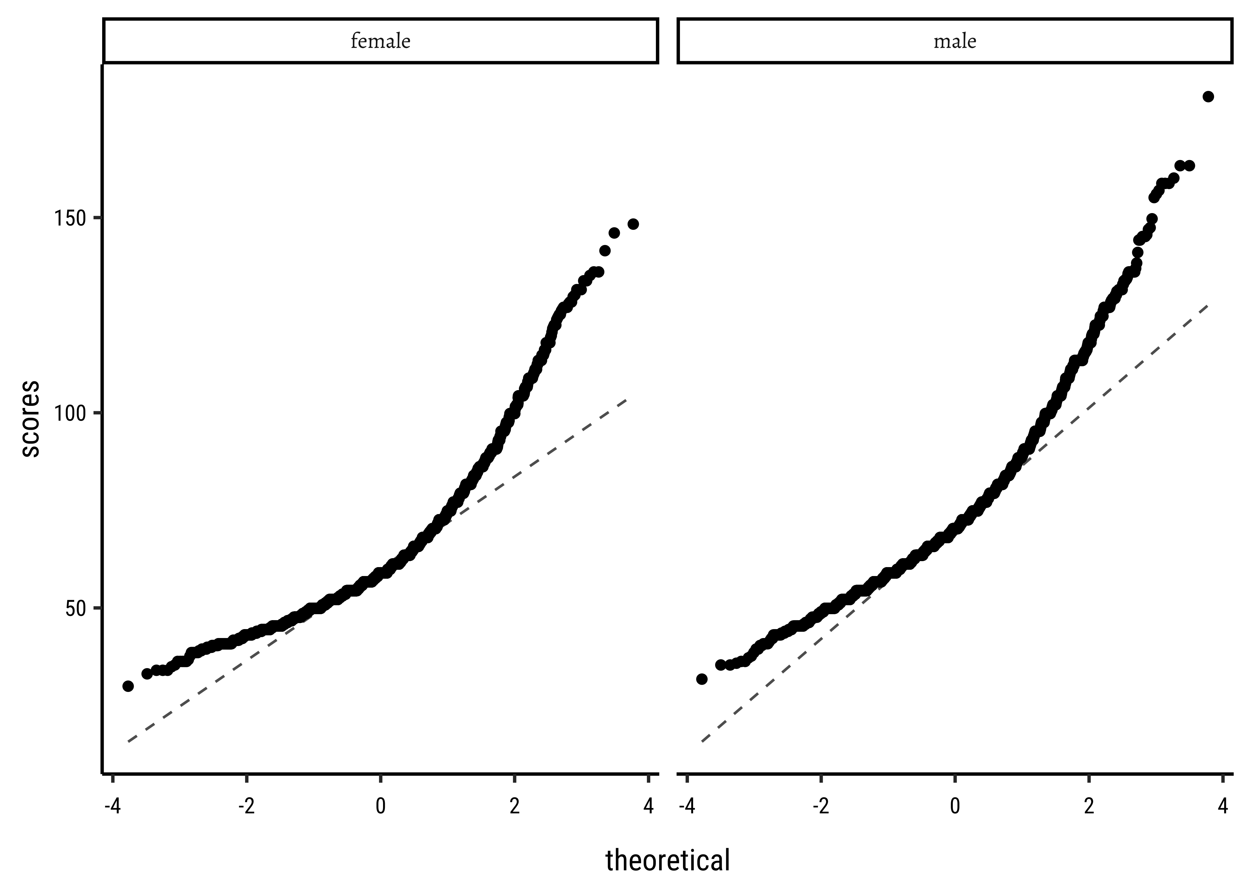
Let us plot frequency distribution and Q-Q plots⁵ for both variables.

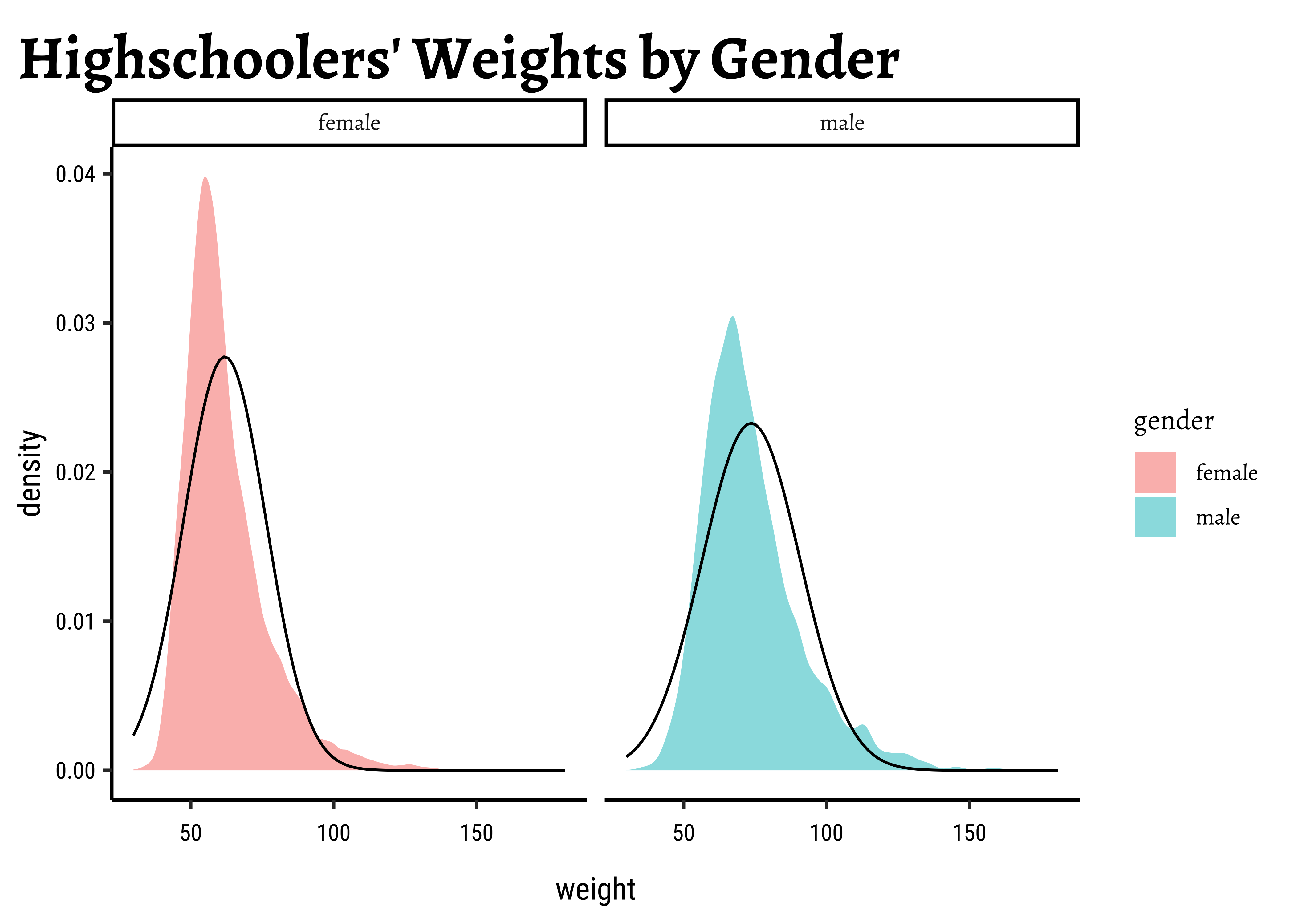
# Set graph theme
theme_set(new = theme_custom())
#
male_student_weights <- yrbss_select_gender %>%
  filter(gender == "male") %>%
  select(weight)
##
female_student_weights <- yrbss_select_gender %>%
  filter(gender == "female") %>%
  select(weight)

# shapiro.test(male_student_weights$weight)
# shapiro.test(female_student_weights$weight)

yrbss_select_gender %>%
  gf_density(~weight,
    fill = ~gender,
    alpha = 0.5,
    title = "Highschoolers' Weights by Gender"
  ) %>%
  gf_facet_grid(~gender) %>%
  gf_fitdistr(dist = "dnorm")
##
yrbss_select_gender %>%
  gf_qqline(~ weight | gender, ylab = "scores") %>%
  gf_qq()

Distributions are not too close to normal…perhaps a hint of a rightward skew, suggesting that there are some obese students.

No real evidence (visually) of the variables being normally distributed.

library(nortest)
nortest::ad.test(male_student_weights$weight)

    Anderson-Darling normality test

data:  male_student_weights$weight
A = 113.23, p-value < 2.2e-16

nortest::ad.test(female_student_weights$weight)

    Anderson-Darling normality test

data:  female_student_weights$weight
A = 157.17, p-value < 2.2e-16

p-values are very low and there is no reason to think that the data is normal.

B. Check for Variances

Let us check if the two variables have similar variances: the var.testdoes this for us, with a NULL hypothesis that the variances are not significantly different:

var.test(weight ~ gender,
  data = yrbss_select_gender,
  conf.int = TRUE,
  conf.level = 0.95
) %>%
  broom::tidy()

# qf(0.975,6164, 6413)

ABCDEFGHIJ0123456789

estimate <dbl>	num.df <int>	den.df <int>	statistic <dbl>	p.value <dbl>	conf.low <dbl>	conf.high <dbl>	method <chr>
0.703976	6164	6413	0.703976	1.065068e-43	0.6700221	0.7396686	F test to compare two variances

1 row | 1-8 of 9 columns

The p.value being so small, we are able to reject the NULL Hypothesis that the variances of weight are nearly equal across the two exercise regimes.

ImportantConditions

1. The two variables are not normally distributed.
2. The two variances are also significantly different.

This means that the parametric t.test must be eschewed in favour of the non-parametric wilcox.test. We will use that, and also attempt linear models with rank data, and a final permutation test.

Observed and Test Statistic

What would be the test statistic we would use? The difference in means. Is the observed difference in the means between the two groups of scores non-zero? We use the diffmean function, from mosaic:

obs_diff_gender <- diffmean(weight ~ gender,
  data = yrbss_select_gender
)

obs_diff_gender

diffmean 
11.70089 

Inference

Using the Mann-Whitney test

Since the data variables do not satisfy the assumption of being normally distributed, and the variances are significantly different, we use the classical wilcox.test, which implements what we need here: the Mann-Whitney U test,

Our model would be:

$$mean(rank(Weigh{t}_{male}))-mean(rank(Weigh{t}_{female}))={\beta }_1;$$

$$H_0:{\mu }_{weight-male}={\mu }_{weight-female}$$

$$H_a:{\mu }_{weight-male}\ne {\mu }_{weight-female}$$

Recall the earlier graph showing ranks of anxiety-scores against Gender.

wilcox.test(weight ~ gender,
  data = yrbss_select_gender,
  conf.int = TRUE,
  conf.level = 0.95
) %>%
  broom::tidy()

ABCDEFGHIJ0123456789

estimate <dbl>	statistic <dbl>	p.value <dbl>	conf.low <dbl>	conf.high <dbl>
-11.33999	10808212	0	-11.34003	-10.87994

1 row | 1-5 of 7 columns

The p.value is negligible and we are able to reject the NULL hypothesis that the means are equal.

Using the Linear Model

We can apply the linear-model-as-inference interpretation to the ranked data data to implement the non-parametric test as a Linear Model:

$$lm(rank(weight)\sim gender)={\beta }_0+{\beta }_1\ast gender$$

$$H_0:{\beta }_1=0$$

$$H_a:{\beta }_1\ne 0$$

# Create a sign-rank function
# signed_rank <- function(x) {sign(x) * rank(abs(x))}

lm(rank(weight) ~ gender,
  data = yrbss_select_gender
) %>%
  broom::tidy(
    conf.int = TRUE,
    conf.level = 0.95
  )

ABCDEFGHIJ0123456789

term <chr>	estimate <dbl>	std.error <dbl>	statistic <dbl>	p.value <dbl>
(Intercept)	4836.157	42.52745	113.71848	0
gendermale	2851.246	59.55633	47.87478	0

2 rows | 1-5 of 7 columns

TipDummy Variables in lm

Note how the Qual variable was used here in Linear Regression lm()! The gender variable was treated as a binary “dummy” variable⁶.

Using the Permutation Test

For the specific data at hand, we need to shuffle the gender and take the test statistic (difference in means) each time.

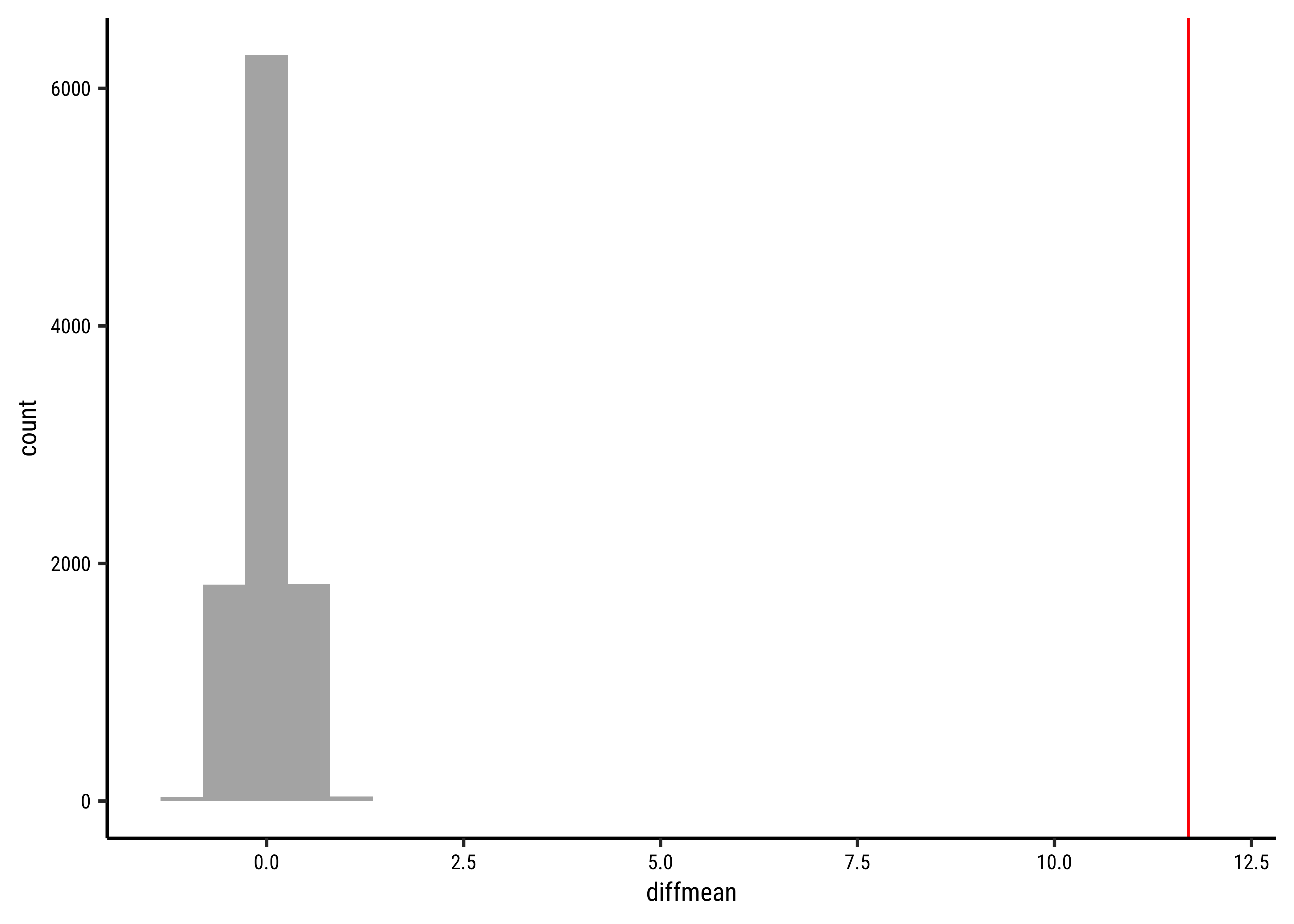
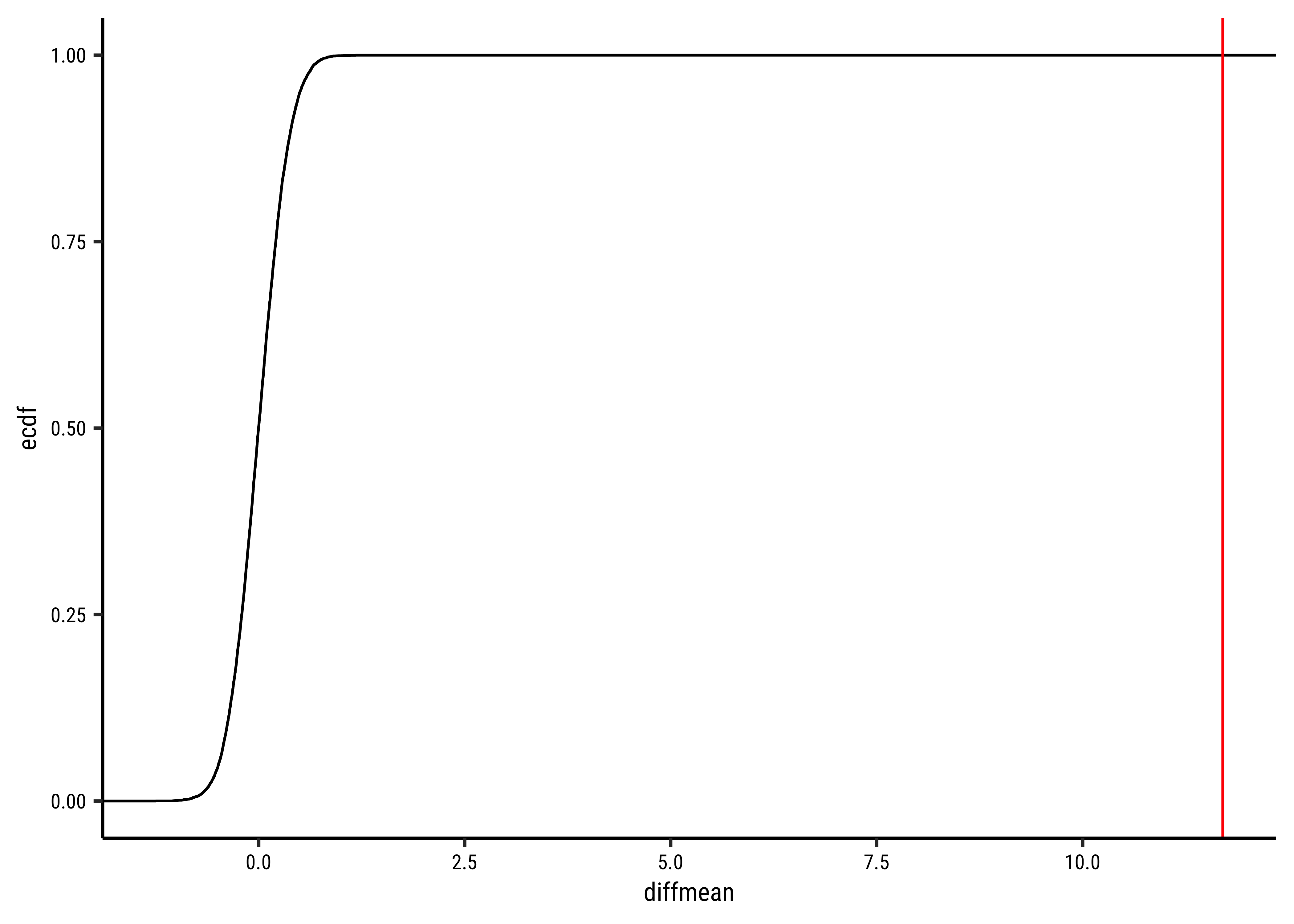
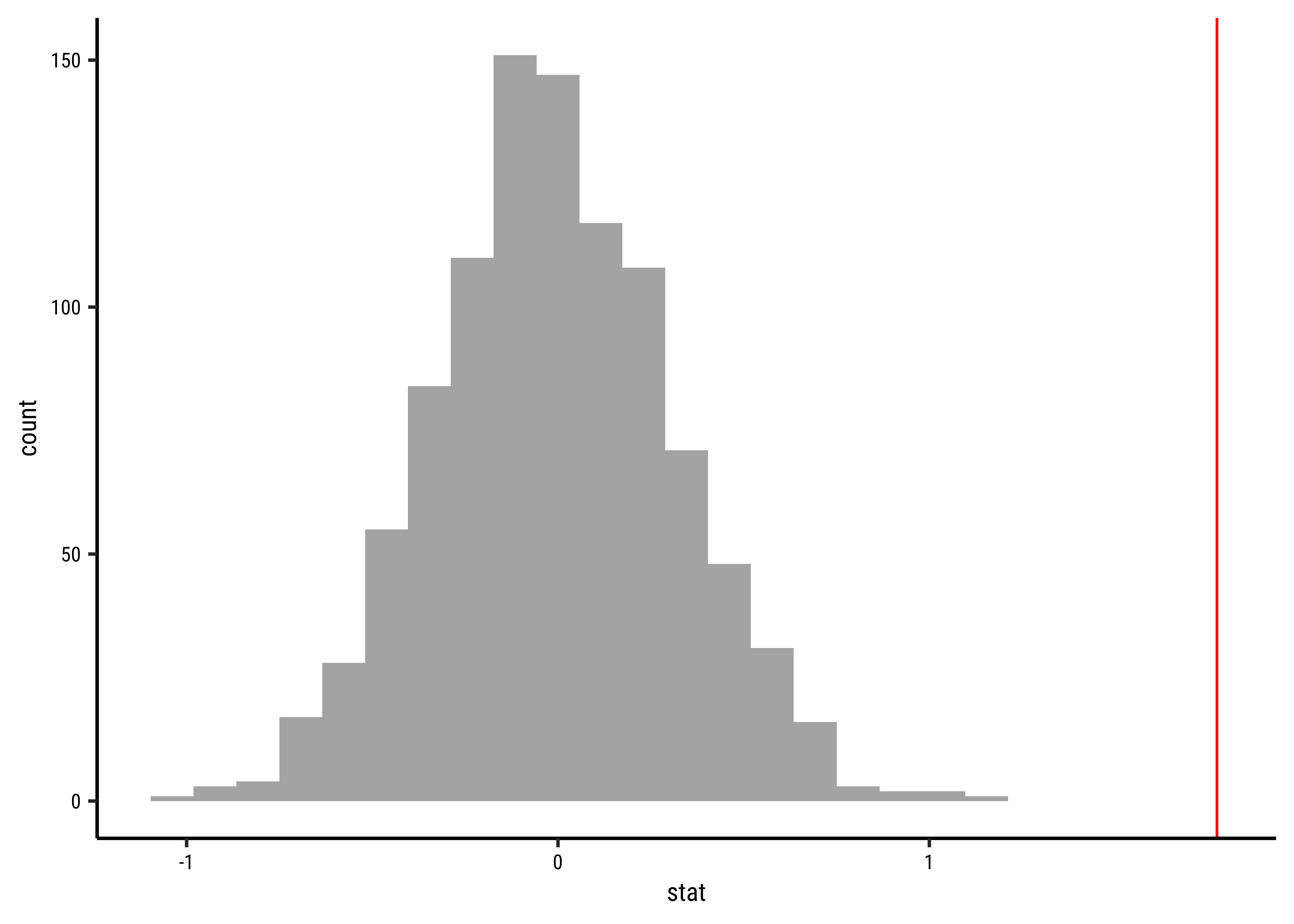
# Set graph theme
theme_set(new = theme_custom())
#
null_dist_weight <-
  do(4999) * diffmean(
    data = yrbss_select_gender,
    weight ~ shuffle(gender)
  )
null_dist_weight
###
prop1(~ diffmean <= obs_diff_gender, data = null_dist_weight)
###
gf_histogram(
  data = null_dist_weight, ~diffmean,
  bins = 25
) %>%
  gf_vline(
    xintercept = obs_diff_gender,
    colour = "red", linewidth = 1,
    title = "Null Distribution by Permutation",
    subtitle = "Histogram"
  ) %>%
  gf_labs(x = "Difference in Means")
###
gf_ecdf(
  data = null_dist_weight, ~diffmean,
  linewidth = 1
) %>%
  gf_vline(
    xintercept = obs_diff_gender,
    colour = "red", linewidth = 1,
    title = "Null Distribution by Permutation",
    subtitle = "Cumulative Density"
  ) %>%
  gf_labs(x = "Difference in Means")

ABCDEFGHIJ0123456789

diffmean <dbl>
0.6371493775
-0.1654355565
-0.2743231230
0.1008648311
0.8977841378
0.3549591481
-0.1142604044
0.1664251413
-1.0260955559
0.4442762828

Next

123456

...

500

Previous

1-10 of 4,999 rows

prop_TRUE 
        1 

Clearly the observed_diff_weight is much beyond anything we can generate with permutations with gender! And hence there is a significant difference in weights across gender!

All Tests Together

We can put all the test results together to get a few more insights about the tests:

wilcox.test(weight ~ gender,
  data = yrbss_select_gender,
  conf.int = TRUE,
  conf.level = 0.95
) %>%
  broom::tidy() %>%
  gt() %>%
  tab_style(
    style = list(cell_fill(color = "cyan"), cell_text(weight = "bold")),
    locations = cells_body(columns = p.value)
  ) %>%
  tab_header(title = "wilcox.test") %>%
  tab_options(table.font.size = 10)

lm(rank(weight) ~ gender,
  data = yrbss_select_gender
) %>%
  broom::tidy(
    conf.int = TRUE,
    conf.level = 0.95
  ) %>%
  gt() %>%
  tab_style(
    style = list(cell_fill(color = "cyan"), cell_text(weight = "bold")),
    locations = cells_body(columns = p.value)
  ) %>%
  tab_header(title = "Linear Model with Ranked Data") %>%
  tab_options(table.font.size = 10)

wilcox.test
estimate	statistic	p.value	conf.low	conf.high	method	alternative
-11.33999	10808212	0	-11.34003	-10.87994	Wilcoxon rank sum test with continuity correction	two.sided

Linear Model with Ranked Data
term	estimate	std.error	statistic	p.value	conf.low	conf.high
(Intercept)	4836.157	42.52745	113.71848	0	4752.797	4919.517
gendermale	2851.246	59.55633	47.87478	0	2734.507	2967.986

The wilcox.test and the linear model with rank data offer the same results. This is of course not surprising!

One Test to Rule Them All: visStatistics again

We need to use a smaller sample of the dataset yrbss_select_gender, for the (same) reason: visstat() defaults to using the shapiro.wilk test internally:

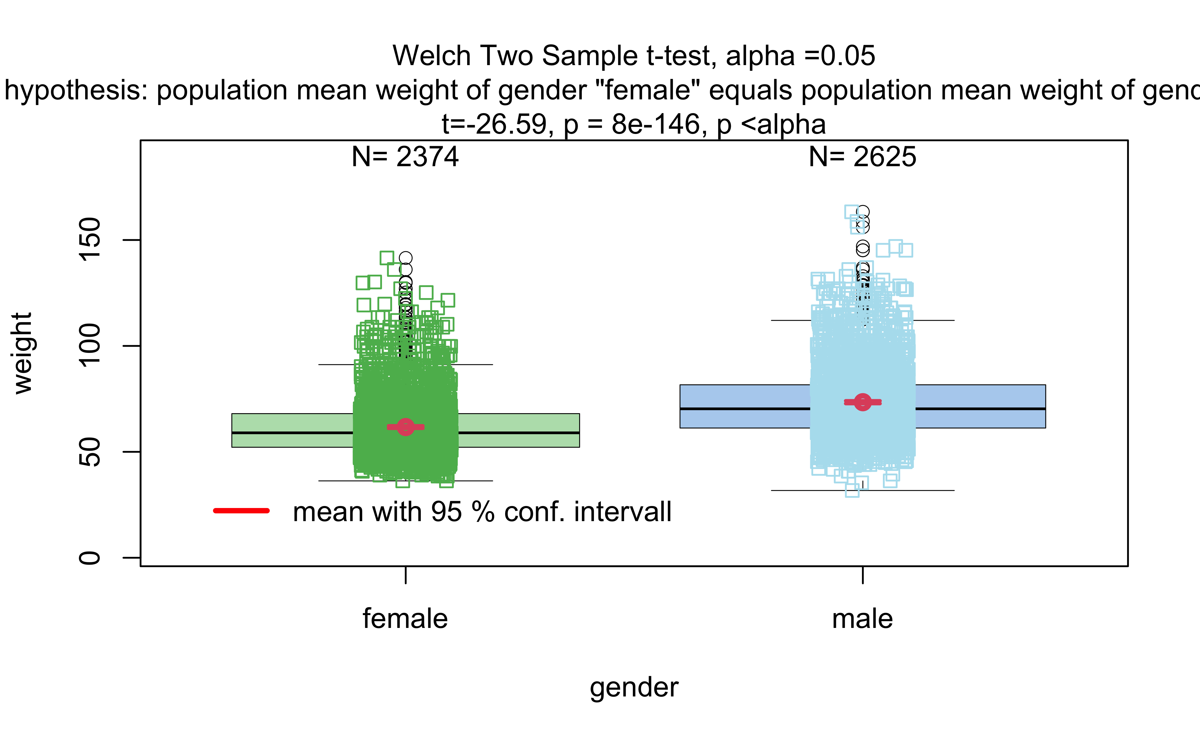
yrbss_select_gender_sample <- yrbss_select_gender %>%
  slice_sample(n = 4999)

visstat(
  x = yrbss_select_gender_sample$gender,
  y = yrbss_select_gender_sample$weight,
  conf.level = 0.95, numbers = TRUE
) %>%
  summary()

Summary of visstat object

--- Named components ---
[1] "dependent variable (response)"    "independent variables (features)"
[3] "t-test-statistics"                "Shapiro-Wilk-test_sample1"       
[5] "Shapiro-Wilk-test_sample2"       

--- Contents ---

$dependent variable (response):
[1] "weight"

$independent variables (features):
[1] male   female
Levels: female male

$t-test-statistics:

    Welch Two Sample t-test

data:  x1 and x2
t = -26.595, df = 4975.1, p-value < 2.2e-16
alternative hypothesis: true difference in means is not equal to 0
95 percent confidence interval:
 -12.59982 -10.86974
sample estimates:
mean of x mean of y 
 61.69867  73.43345 


$Shapiro-Wilk-test_sample1:

    Shapiro-Wilk normality test

data:  x
W = 0.90106, p-value < 2.2e-16


$Shapiro-Wilk-test_sample2:

    Shapiro-Wilk normality test

data:  x
W = 0.93466, p-value < 2.2e-16


--- Attributes ---
$plot_paths
character(0)

Compare these results with those calculated earlier!

Case Study #3: Weight vs Exercise in the YRBSS Survey

Finally, consider the possible relationship between a highschooler’s weight and their physical activity.

First, let’s create a new variable physical_3plus, which will be coded as either “yes” if the student is physically active for at least 3 days a week, and “no” if not. Recall that we have several missing data in that column, so we will (sadly) drop these before generating the new variable:

yrbss_select_phy <- yrbss %>%
  drop_na(physically_active_7d, weight) %>%
  ## add new variable physical_3plus
  mutate(
    physical_3plus = if_else(physically_active_7d >= 3,
      "yes", "no"
    ),
    # Convert it to a factor Y/N
    physical_3plus = factor(physical_3plus,
      labels = c("yes", "no"),
      levels = c("yes", "no")
    )
  ) %>%
  select(weight, physical_3plus)

# Let us check
yrbss_select_phy %>% count(physical_3plus)

ABCDEFGHIJ0123456789

physical_3plus <fct>	n <int>
yes	8342
no	4022

2 rows

NoteResearch Question

Does weight vary based on whether students exercise on more or less than 3 days a week? (physically_active_7d >= 3 days)

Inspecting and Charting Data

We can make distribution plots for weight by physical_3plus:

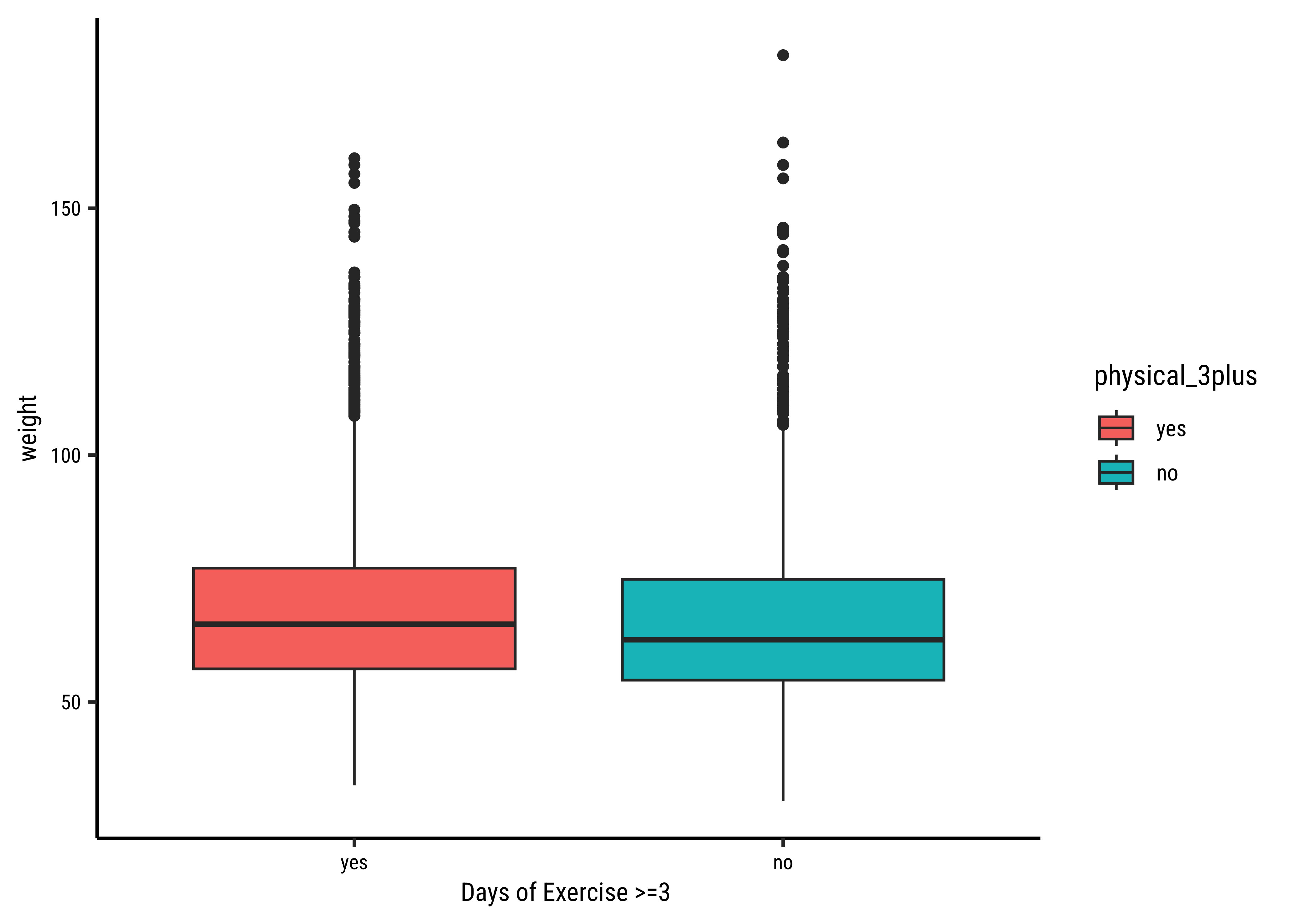
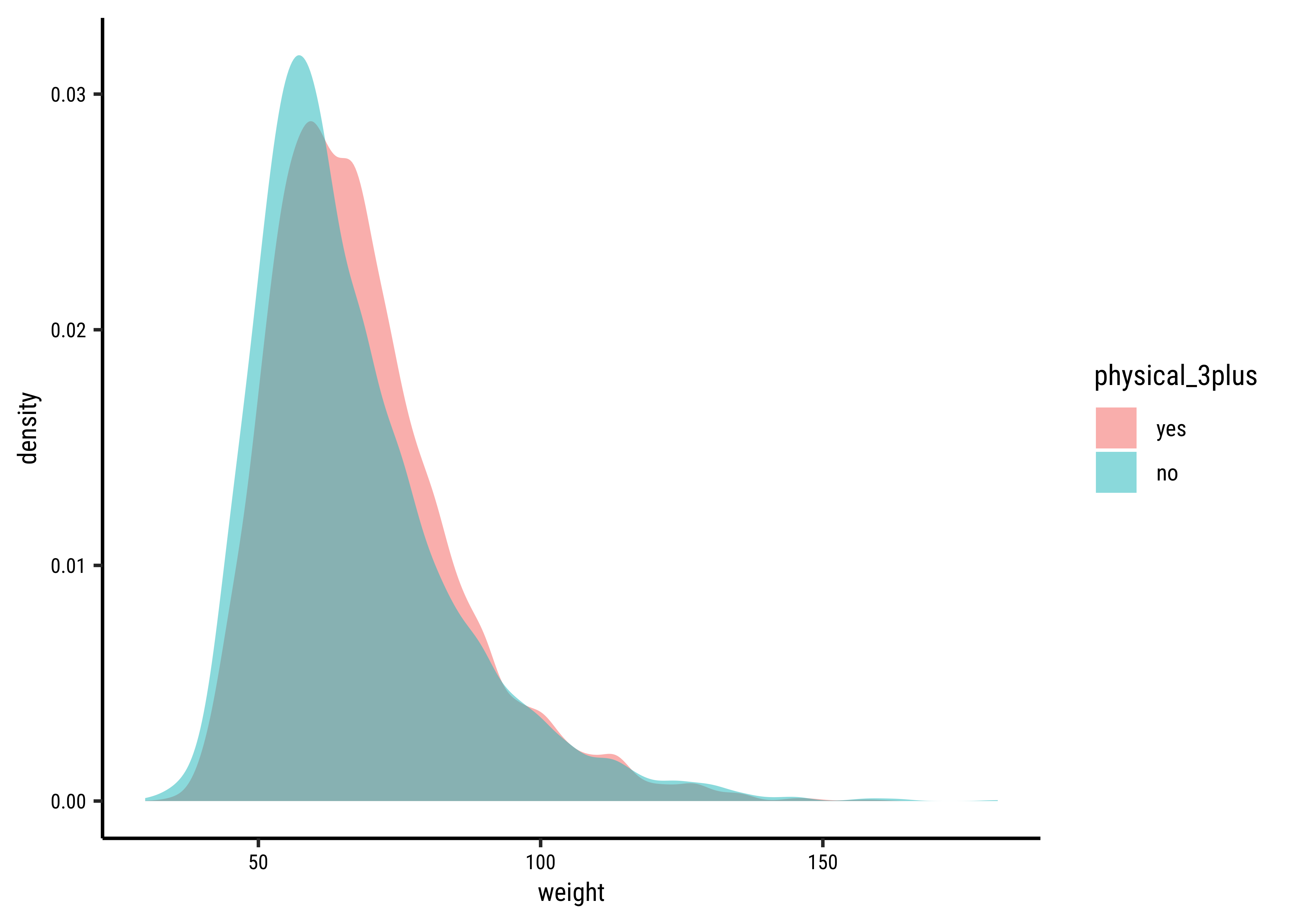
# Set graph theme
theme_set(new = theme_custom())
###
yrbss_select_phy %>%
  gf_jitter(weight ~ physical_3plus,
    group = ~physical_3plus,
    width = 0.08, alpha = 0.08,
    xlab = "Days of Exercise >=3"
  ) %>%
  gf_summary(
    geom = "point", size = 3, group = ~physical_3plus,
    colour = ~physical_3plus
  ) %>%
  gf_line(
    group = 1, # weird remedy to fix groups error message!
    stat = "summary", linewidth = 1,
    geom = "line", colour = ~"MeanDifferenceLine"
  )
###
gf_density(~weight,
  fill = ~physical_3plus,
  data = yrbss_select_phy
)

The jitter and density plots show the comparison between the two means. We can also compare the means of the distributions using the following to first group the data by the physical_3plus variable, and then calculate the mean weight in these groups using the mean function while ignoring missing values by setting the na.rm argument to TRUE.

yrbss_select_phy %>%
  group_by(physical_3plus) %>%
  summarise(mean_weight = mean(weight, na.rm = TRUE))

ABCDEFGHIJ0123456789

physical_3plus <fct>	mean_weight <dbl>
yes	68.44847
no	66.67389

2 rows

There is an observed difference, but is this difference large enough to deem it “statistically significant”? In order to answer this question we will conduct a hypothesis test. But before that a few more checks on the data:

A. Check for Normality

As stated before, statistical tests for means usually require a couple of checks:

• Are the data normally distributed?
  
• Are the data variances similar?

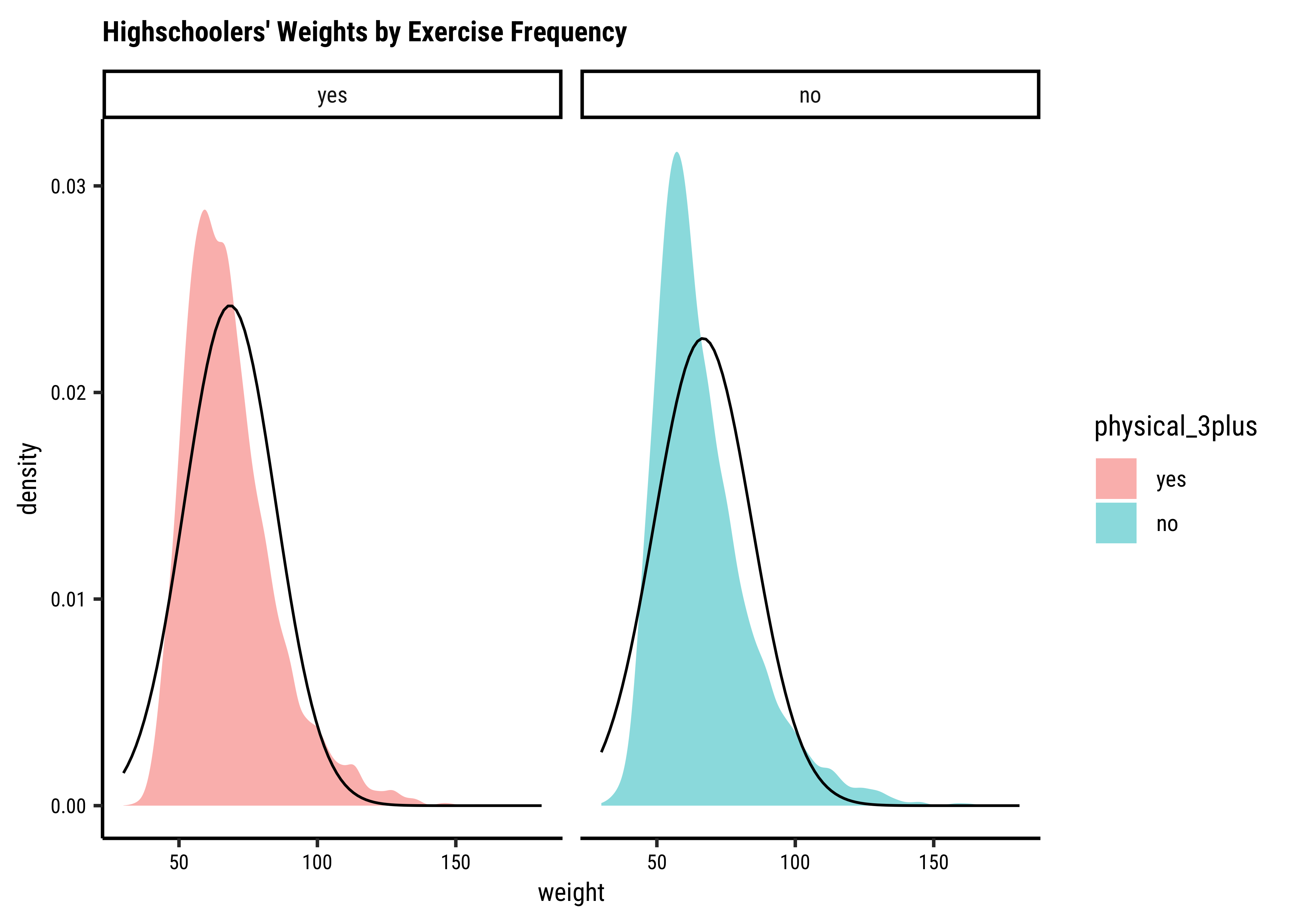
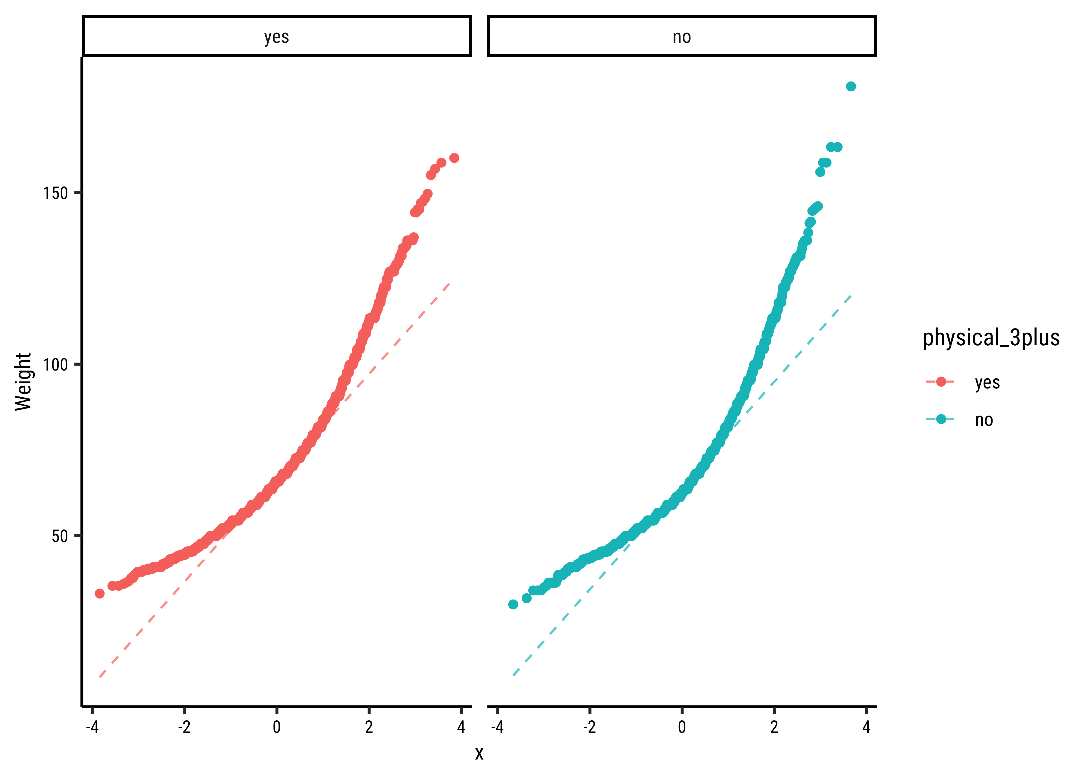
Let us also complete a visual check for normality,with plots since we cannot do a shapiro.test:

# Set graph theme
theme_set(new = theme_custom())
#
yrbss_select_phy %>%
  gf_density(~weight,
    fill = ~physical_3plus,
    alpha = 0.5,
    title = "Highschoolers' Weights by Exercise Frequency"
  ) %>%
  gf_facet_grid(~physical_3plus) %>%
  gf_fitdistr(dist = "dnorm")
##
yrbss_select_phy %>%
  gf_qq(~ weight | physical_3plus,
    color = ~physical_3plus
  ) %>%
  gf_qqline(ylab = "Weight")

Again, not normally distributed…

B. Check for Variances

Let us check if the two variables have similar variances: the var.test does this for us, with a NULL hypothesis that the variances are not significantly different:

var.test(weight ~ physical_3plus,
  data = yrbss_select_phy,
  conf.int = TRUE,
  conf.level = 0.95
) %>%
  broom::tidy()

# Critical F value
qf(0.975, 4021, 8341)

ABCDEFGHIJ0123456789

estimate <dbl>	num.df <int>	den.df <int>	statistic <dbl>	p.value <dbl>	conf.low <dbl>	conf.high <dbl>
0.8728201	8341	4021	0.8728201	4.390179e-07	0.8273749	0.9202997

1 row | 1-7 of 9 columns

[1] 1.054398

The p.value states the probability of the data being what it is, assuming the NULL hypothesis that variances were similar. It being so small, we are able to reject this NULL Hypothesis that the variances of weight are nearly equal across the two exercise frequencies. (Compare the statistic in the var.test with the critical F-value)

ImportantConditions

1. The two variables are not normally distributed.
2. The two variances are also significantly different.

Hence we will have to use non-parametric tests to infer if the means are similar.

Hypothesis

Based on the graphs, how would we formulate our Hypothesis? We wish to infer whether there is difference in mean weight across physical_3plus. So accordingly:

$$H_0:{\mu }_{physical-3plus-Yes}={\mu }_{physical-3plus-No}$$

$$H_a:{\mu }_{physical-3plus-Yes}\ne {\mu }_{physical-3plus-No}$$

Observed and Test Statistic

What would be the test statistic we would use? The difference in means. Is the observed difference in the means between the two groups of scores non-zero? We use the diffmean function, from mosaic:

obs_diff_phy <- diffmean(weight ~ physical_3plus,
  data = yrbss_select_phy
)

obs_diff_phy

 diffmean 
-1.774584 

Inference

Using parametric t.test

Well, the variables are not normally distributed, and the variances are significantly different so a standard t.test is not advised. We can still try:

mosaic::t_test(weight ~ physical_3plus,
  var.equal = FALSE, # Welch Correction
  data = yrbss_select_phy
) %>%
  broom::tidy()

ABCDEFGHIJ0123456789

estimate <dbl>	estimate1 <dbl>	estimate2 <dbl>	statistic <dbl>	p.value <dbl>	parameter <dbl>	conf.low <dbl>	conf.high <dbl>
1.774584	68.44847	66.67389	5.353003	8.907531e-08	7478.84	1.124728	2.424441

1 row | 1-8 of 10 columns

The p.value is $8.9e-08$ ! And the Confidence Interval is clear of $0$. So the t.test gives us good reason to reject the Null Hypothesis that the means are similar. But can we really believe this, given the non-normality of data?

Using non-parametric paired Wilcoxon test

However, we have seen that the data variables are not normally distributed. So a Wilcoxon Test, using signed-ranks, is indicated: (recall the model!)

# For stability reasons, it may be advisable to use rounded data or to set digits.rank = 7, say,
# such that determination of ties does not depend on very small numeric differences (see the example).

wilcox.test(weight ~ physical_3plus,
  conf.int = TRUE,
  conf.level = 0.95,
  data = yrbss_select_phy
) %>%
  broom::tidy()

ABCDEFGHIJ0123456789

estimate <dbl>	statistic <dbl>	p.value <dbl>	conf.low <dbl>	conf.high <dbl>
2.269967	18314392	1.262977e-16	1.819992	2.720077

1 row | 1-5 of 7 columns

The nonparametric wilcox.test also suggests that the means for weight across physical_3plus are significantly different.

Using the Linear Model Interpretation

We can apply the linear-model-as-inference interpretation to the ranked data data to implement the non-parametric test as a Linear Model:

$$\begin{gathered} lm(rank(weight)\sim physical.3plus)={\beta }_0+{\beta }_1\times physical.3plus \\ {H}_0:{\beta }_1=0 \\ {H}_a:{\beta }_1\ne 0 \end{gathered}$$

lm(rank(weight) ~ physical_3plus,
  data = yrbss_select_phy
) %>%
  broom::tidy(
    conf.int = TRUE,
    conf.level = 0.95
  )

ABCDEFGHIJ0123456789

term <chr>	estimate <dbl>	std.error <dbl>	statistic <dbl>	p.value <dbl>
(Intercept)	6366.9438	38.96362	163.407391	0.000000e+00
physical_3plusno	-566.9972	68.31527	-8.299715	1.151496e-16

2 rows | 1-5 of 7 columns

Here too, the linear model using rank data arrives at a conclusion similar to that of the Mann-Whitney U test.

Using Permutation Tests

For this last Case Study, we will do this in two ways, just for fun: one using our familiar mosaic package, and the other using the package infer.

But first, we need to initialize the test, which we will save as obs_diff_**.

obs_diff_infer <- yrbss_select_phy %>%
  infer::specify(weight ~ physical_3plus) %>%
  infer::calculate(
    stat = "diff in means",
    order = c("yes", "no")
  )
obs_diff_infer
##
obs_diff_mosaic <-
  mosaic::diffmean(~ weight | physical_3plus,
    data = yrbss_select_phy
  )
obs_diff_mosaic
##
obs_diff_phy

ABCDEFGHIJ0123456789

stat <dbl>
1.774584

1 row

 diffmean 
-1.774584 

 diffmean 
-1.774584 

Important

Note that obs_diff_infer is a 1 X 1 dataframe; obs_diff_mosaic is a scalar!!

Using infer

Next, we will work through creating a permutation distribution using tools from the infer package.

In infer, the specify() function is used to specify the variables you are considering (notated y ~ x), and you can use the calculate() function to specify the statistic you want to calculate and the order of subtraction you want to use. For this hypothesis, the statistic you are searching for is the difference in means, with the order being yes - no.

After you have calculated your observed statistic, you need to create a permutation distribution. This is the distribution that is created by shuffling the observed weights into new physical_3plus groups, labeled “yes” and “no”.

We will save the permutation distribution as null_dist.

null_dist <- yrbss_select_phy %>%
  specify(weight ~ physical_3plus) %>%
  hypothesize(null = "independence") %>%
  generate(reps = 999, type = "permute") %>%
  calculate(
    stat = "diff in means",
    order = c("yes", "no")
  )
null_dist

ABCDEFGHIJ0123456789

replicate <int>	stat <dbl>
1	0.4821793257
2	0.0856206574
3	-0.2282522195
4	-0.1363242510
5	-0.0343286481
6	-0.9326512912
7	-0.0180811369
8	-0.1961588708
9	-0.2009568430
10	-0.3252545410

Next

12345

...

100

Previous

1-10 of 999 rows

The hypothesize() function is used to declare what the null hypothesis is. Here, we are assuming that student’s weight is independent of whether they exercise at least 3 days or not.

We should also note that the type argument within generate() is set to "permute". This ensures that the statistics calculated by the calculate() function come from a reshuffling of the data (not a resampling of the data)! Finally, the specify() and calculate() steps should look familiar, since they are the same as what we used to find the observed difference in means!

We can visualize this null distribution with the following code:

# Set graph theme
theme_set(new = theme_custom())
#
null_dist %>%
  visualise() + # Note this plus sign!
  shade_p_value(obs_diff_infer,
    direction = "two-sided"
  )

Now that you have calculated the observed statistic and generated a permutation distribution, you can calculate the p-value for your hypothesis test using the function get_p_value() from the infer package.

null_dist %>%
  get_p_value(
    obs_stat = obs_diff_infer,
    direction = "two_sided"
  )

ABCDEFGHIJ0123456789

p_value <dbl>
0

1 row

What warning message do you get? Why do you think you get this warning message? Let us construct and record a confidence interval for the difference between the weights of those who exercise at least three times a week and those who don’t, and interpret this interval in context of the data.

null_dist %>%
  infer::get_confidence_interval(
    point_estimate = obs_diff_infer,
    level = 0.95
  )

ABCDEFGHIJ0123456789

lower_ci <dbl>	upper_ci <dbl>
-0.6152689	0.6082389

1 row

It does look like the observed_diff_infer is too far away from this confidence interval. Hence if there was no difference in weight caused by physical_3plus, we would never have observed it! Hence the physical_3plus does have an effect on weight!

Using mosaic

We already have the observed difference, obs_diff_mosaic. Now we generate the null distribution using permutation, with mosaic:

null_dist_mosaic <- do(999) *
  diffmean(~ weight | shuffle(physical_3plus),
    data = yrbss_select_phy
  )

We can also generate the histogram of the null distribution, compare that with the observed diffrence and compute the p-value and confidence intervals:

# Set graph theme
theme_set(new = theme_custom())
#
gf_histogram(~diffmean, data = null_dist_mosaic) %>%
  gf_vline(
    xintercept = obs_diff_mosaic,
    colour = "red", linewidth = 2
  )

# p-value
prop(~ diffmean != obs_diff_mosaic, data = null_dist_mosaic)

prop_TRUE 
        1 

# Confidence Intervals for p = 0.95
mosaic::cdata(~diffmean, p = 0.95, data = null_dist_mosaic)

ABCDEFGHIJ0123456789

	lower <dbl>	upper <dbl>	central.p <dbl>
2.5%	-0.6788335	0.6112242	0.95

1 row

Again, it does look like the observed_diff_infer is too far away from this NULL distribution. Hence if there was no difference in weight caused by physical_3plus, we would never have observed it! Hence the physical_3plus does have an effect on weight!

Clearly there is a serious effect of Physical Exercise on the body weights of students in the population from which this dataset is drawn.

Wait, But Why?

• We need often to infer differences in means between Quantitative variables in a Population
• We treat our dataset as a sample from the population, which we cannot access
• We can apply all the CLT ideas +t.test if the two variables in the dataset satisfy the conditions of normality, equal variance
• Else use non-parametric wilcox.test
• And by treating the two variables as one Quant in two groups, we can simply perform a Permutation test

Conclusion

• We have learnt how to perform inference for independent means.
  
• We have looked at the conditions that make the regular t.test possible, and learnt what to do if the conditions of normality and equal variance are not met.
  
• We have also looked at how these tests can be understood as manifestations of the linear model, with data and sign-ranked data.
  

Your Turn

1. Try the SwimRecords dataset from the mosaicData package.

2. Try some of the datasets in the moderndive package. Install it , peasants. And type in your Console data(package = "moderndive") to see what you have. Teacher evals might interest you!

References

1. Randall Pruim, Nicholas J. Horton, Daniel T. Kaplan, Start Teaching with R
2. https://bcs.wiley.com/he-bcs/Books?action=index&itemId=111941654X&bcsId=11307
3. https://statsandr.com/blog/wilcoxon-test-in-r-how-to-compare-2-groups-under-the-non-normality-assumption/

R Package Citations

Package	Version	Citation
explore	1.3.4	@explore
infer	1.0.8	@infer
openintro	2.5.0	@openintro
resampledata	0.3.2	@resampledata
TeachHist	0.2.1	@TeachHist
TeachingDemos	2.13	@TeachingDemos
visStatistics	0.1.7	@visStatistics

Footnotes

1. https://stats.stackexchange.com/questions/2492/is-normality-testing-essentially-useless

2. https://www.allendowney.com/blog/2023/01/28/never-test-for-normality/

3. https://stats.stackexchange.com/q/113337

4. https://www.middleprofessor.com/files/applied-biostatistics_bookdown/_book/intro-linear-models.html#a-linear-model-can-be-fit-to-data-with-continuous-discrete-or-categorical-x-variables

5. https://stats.stackexchange.com/questions/92374/testing-large-dataset-for-normality-how-and-is-it-reliable

6. https://en.wikipedia.org/wiki/Dummy_variable_(statistics)