Affine Transformation Fractals

Created in Translation

Iterated Functions

Fractals

Affine Transformations

Barnsley

Published

January 28, 2025

Modified

May 17, 2025

Inspiration

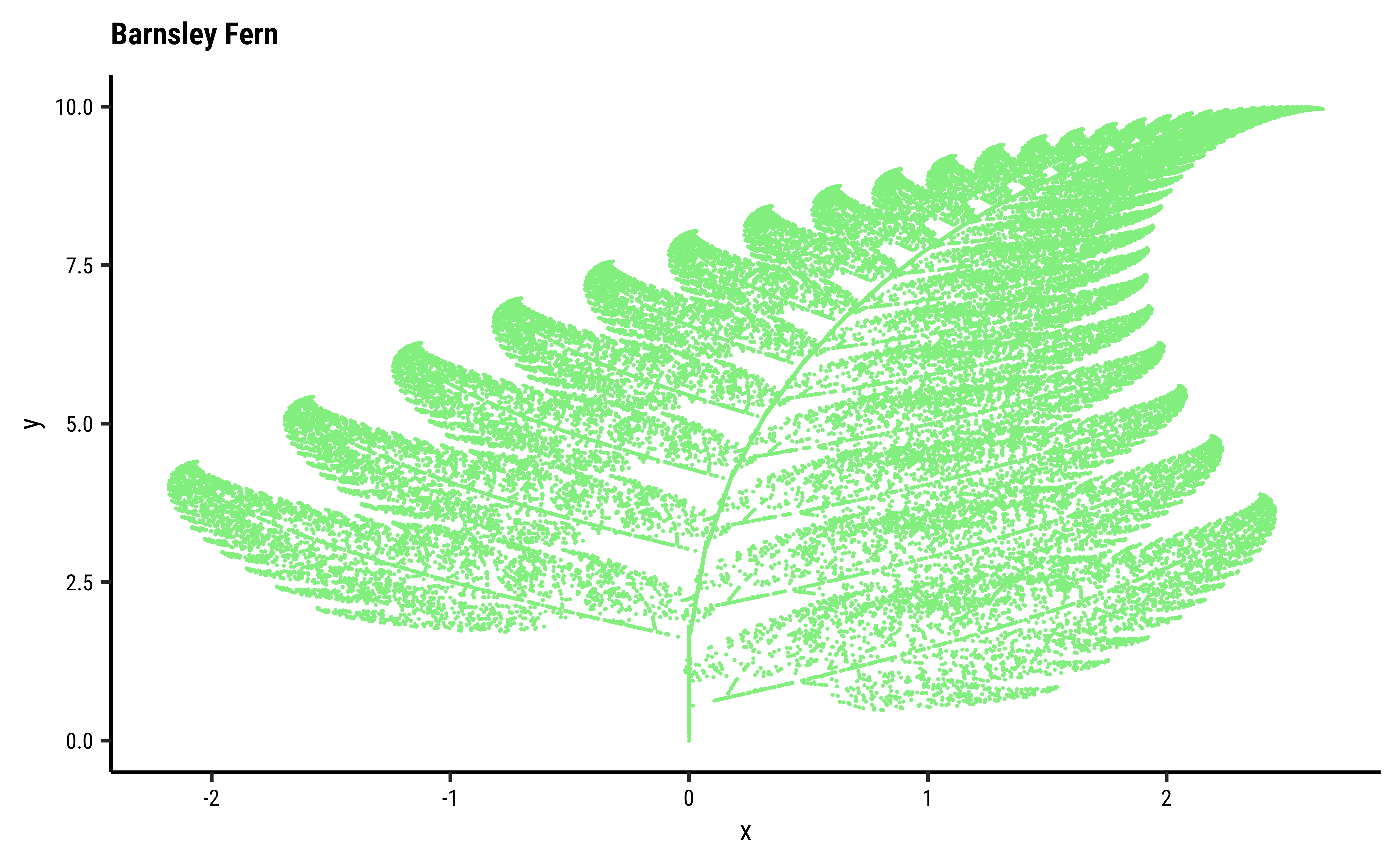
This is a mathematically created fern! It uses, (gasp!) repeated matrix multiplication and addition!

We’ll see.

Introduction

The self-similarity of fractals suggests that we could create new fractals from a basic shape using the following procedure:

Start with a basic shape, e.g. a rectangle
Define a set of transformations: scaling / mirroring / translation / combination (say n scaled+rotated replicates)
Run these transformations on the basic shape
Feed the output back to the input ( Classic IFR )
Wait for the pattern to emerge.

See the figure below to get an idea of this process.

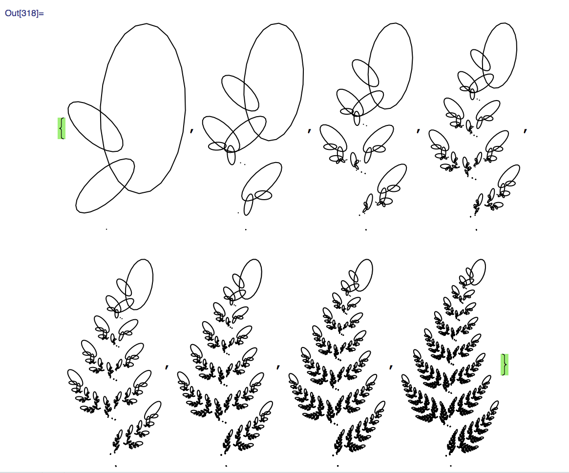
Well, this works, provided the transformations include significant amounts of scaling (i.e. reduction in size). You can imagine that if the basic shape does not shrink fast enough, the pattern converges very slowly and would remain chunky even after a large number of iterations.

Secondly, the number of operations quickly becomes exponentially high, as each stage creates n-fold computation increase. Indeed, if we run $d$ iterations, then the computations scale as $n^{d}$ , which can very quickly become out of hand!!

So what to do? Just like with the DeepSeek-R1 algorithm that simplified a great deal of AI algorithms, we have recourse to what is called the Barnsley Algorithm. NOTE: especially note the terrific pictures on this stackexchange page!

First let us understand what are Affine Transformations and then build our fractals.

What is an Affine Transformation?

Affine Transformations are defined as a transformations of a space that are:

linear (no nonlinear functions of an x-coordinate, say $e^{x}$ )
reversible.

Affine transformations can be represented by matrices which multiply the coordinates of a shape in space. Multiple transformations can be understood a series of matrix multiplications, and can indeed be collapsed into a SINGLE matrix multiplication of the coordinates of the shape.

See this webpage at Mathigon to get an idea of rigid transformations of shape.

Some Examples of Affine Transformations

Here are some short videos of affine transformations:

Video Player is loading.

Current Time 0:00

Duration 0:20

Loaded: 100.00%

Stream Type LIVE

Remaining Time 0:20

Figure 2: Scaling Along X

Video Player is loading.

Current Time 0:00

Duration 0:20

Loaded: 100.00%

Stream Type LIVE

Remaining Time 0:20

Figure 3: Scaling Along Y

Video Player is loading.

Current Time 0:00

Duration 0:20

Loaded: 100.00%

Stream Type LIVE

Remaining Time 0:20

Figure 4: Shearing Along X

Video Player is loading.

Current Time 0:00

Duration 0:20

Loaded: 100.00%

Stream Type LIVE

Remaining Time 0:20

Figure 5: Shearing Along Y

Video Player is loading.

Current Time 0:00

Duration 0:20

Loaded: 100.00%

Stream Type LIVE

Remaining Time 0:20

Figure 6: Translation Along X

Video Player is loading.

Current Time 0:00

Duration 0:20

Loaded: 100.00%

Stream Type LIVE

Remaining Time 0:20

Figure 7: Translation Along Y

Designing with Affine Transformations

So how do we use these Affine Transformations? Let us paraphrase what Gary William Flake says in his book The Computational Beauty of Nature:

If $p$ is a point in space, and its affine transformation(s) is $L (p$ ), then:

If $p$ is on the final fractal, then so is $L (p)$ ;
If $p$ is not part of the final fractal, then $L (p)$ will be atleast closer to the final fractal than $p$ itself.

These ideas give us our final algorithm for designing a fractal with affine transformations.

Start with any point $p$
Pick a (set of) Affine transformations $L_{i} (p)$ that allow us to imagine the final shape
Take the affine transformation $L_{i} (p)$ of point $p$ . Choose $i$ at random!
Use an IFR: pipe the result back into the input
Make a large number of iterations
Plot all intermediate points that come out of the IFR

With this approach, the points rapidly land up on the fractal which builds up over multiple iterations. We can start anywhere in space and it will still converge.

The additional feature of the Barnsley algorithm is the randomness: since most fractals use not one but several affine transformations to create a multiplicity of forms, at each iteration we can randomly choose between them!

The block diagram of the Barnsley Algorithm looks like this:

Using p5.js
Using R

How to understand this sketch? Here is Dan Shiffman again!

In the code below, the Affine transformations $A f_{i}$ are of the form

$\begin{matrix} (1) & A F_{i} = A_{i} * X + B_{i}, i = 1. . .4 \end{matrix}$

with four options each for matrix $A$ and matrix $B$ , and $X = (x, y)$ , the current point coordinates (seed input, then output feedback for recursion). There are 50000 iterations performed and at each interation, a random A and a random B are picked to provide the Affine Transformation for that iteration.

The starting “seed point” is simply $X = (0, 0)$ .

The probabilities with which each affine transformation is chosen are not all equal; these can be tweaked to see the effect on the fractal.

The four options for the $A_{i}$ matrices are:

Show the Code

A <- vector(mode = "list", length = 4)
# Four Affine translation Matrices
A[[1]] <- matrix(c(0, 0, 0, 0.18), nrow = 2)
A[[2]] <- matrix(c(0.85, -0.04, 0.04, 0.85), nrow = 2)
A[[3]] <- matrix(c(0.2, 0.23, -0.26, 0.22), nrow = 2)
A[[4]] <- matrix(c(-0.15, 0.36, 0.28, 0.24), nrow = 2)
as_sym(A[[1]])
as_sym(A[[2]])
as_sym(A[[3]])
as_sym(A[[4]])

c: ⎡0   0  ⎤
   ⎢       ⎥
   ⎣0  0.18⎦
c: ⎡0.85   0.04⎤
   ⎢           ⎥
   ⎣-0.04  0.85⎦
c: ⎡0.2   -0.26⎤
   ⎢           ⎥
   ⎣0.23  0.22 ⎦
c: ⎡-0.15  0.28⎤
   ⎢           ⎥
   ⎣0.36   0.24⎦

[\begin{matrix} 0.00 & 0.00 \\ 0.00 & 0.18 \end{matrix}]

$$ {#eq-A1}

[\begin{matrix} 0.85 & 0.04 \\ - 0.04 & 0.85 \end{matrix}]

[\begin{matrix} 0.20 & - 0.26 \\ 0.23 & 0.22 \end{matrix}]

[\begin{matrix} - 0.15 & 0.28 \\ 0.36 & 0.24 \end{matrix}]

$\begin{matrix} (2) & X = U Λ V \end{matrix}$

[\begin{matrix} 0.00 & 0.00 \\ 0.00 & 0.18 \end{matrix}]

$$ {#eq-A1}

And the four options for the $B_{i}$ matrices are:

Show the Code

# Four Simple translation Matrices
b <- vector(mode = "list", length = 4)
b[[1]] <- matrix(c(0, 0))
b[[2]] <- matrix(c(0, 1.6))
b[[3]] <- matrix(c(0, 1.6))
b[[4]] <- matrix(c(0, 0.54))
as_sym(b[[1]])
as_sym(b[[2]])
as_sym(b[[3]])
as_sym(b[[4]])

c: [0  0]ᵀ
c: [0  1.6]ᵀ
c: [0  1.6]ᵀ
c: [0  0.54]ᵀ

By randomly choosing any of the $16$ resulting transformations, with different but fixed probablilities, we compute and render the Barnsley fern:

Show the Code

# Iteratively build the fern
theme_set(theme_custom())
#
n <- 50000
x <- numeric(n)
y <- numeric(n)
x[1] <- 0
y[1] <- 0 # Starting point (0,0). Can be anything!

for (i in 1:(n - 1)) {
  # Randomly sample the 4 + 4 translations based on a probability
  # Change these to try different kinds of ferns
  trans <- sample(1:4, prob = c(.02, .9, .09, .08), size = 1)

  # Translate **current** xy based on the selected translation
  # Apply one of 16 possible affine transformations
  xy <- A[[trans]] %*% c(x[i], y[i]) + b[[trans]]
  x[i + 1] <- xy[1] # Save x component
  y[i + 1] <- xy[2] # Save y component
}
# Plot this baby
# plot(y,x,col= "pink",cex=0.1)
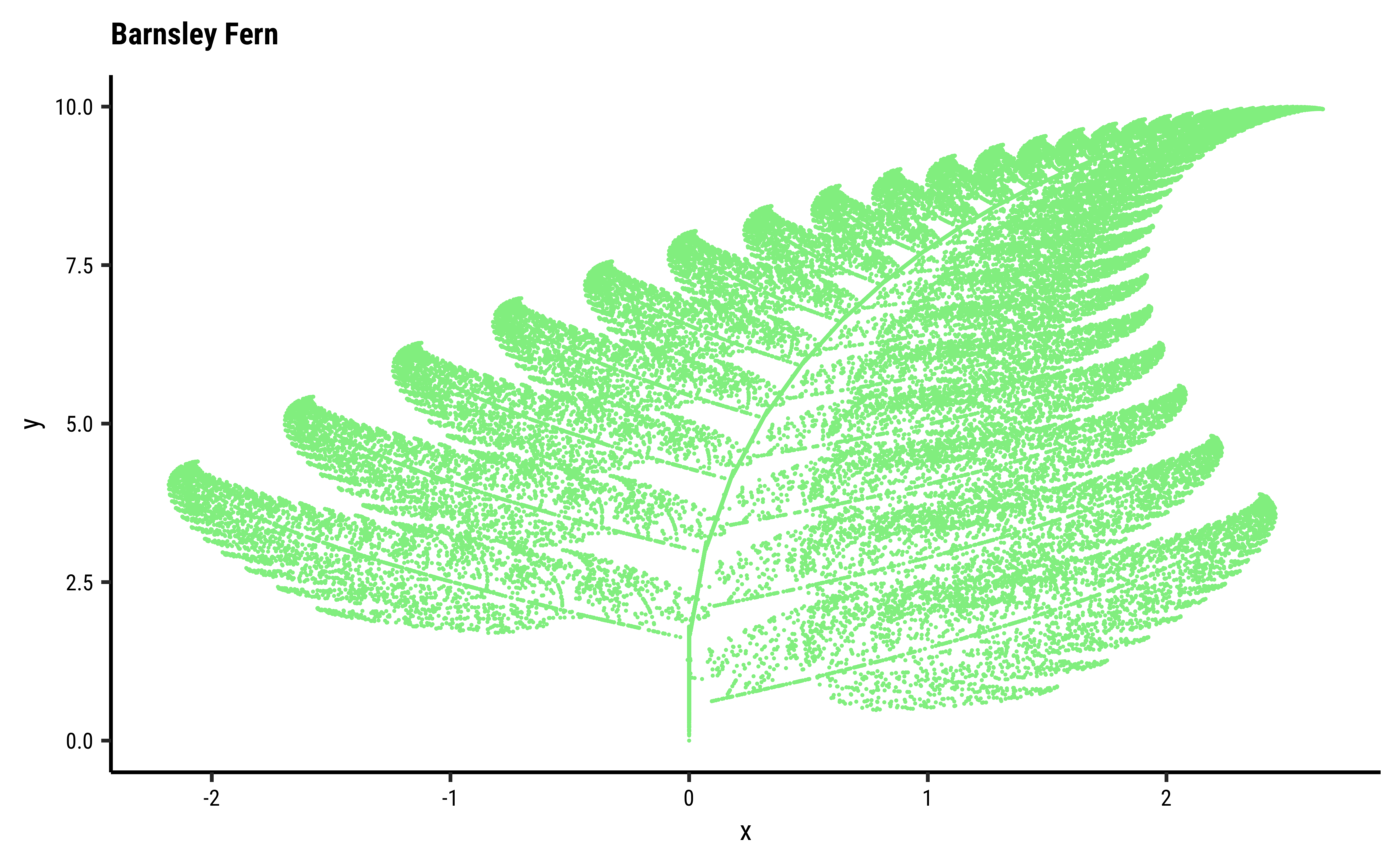
gf_point(y ~ x,
  colour = "lightgreen", size = 0.02,
  title = "Barnsley Fern"
)

Show the Code

X <- matrix(c(5, 5), nrow = 2)
as_sym(A[[1]])
as_sym(X)
as_sym(A[[1]]) %*% as_sym(X)

c: ⎡0   0  ⎤
   ⎢       ⎥
   ⎣0  0.18⎦
c: [5  5]ᵀ
c: [0  0.9]ᵀ

Vertical movement with Shrinkage

Show the Code

X <- matrix(c(5, 5), nrow = 2)
as_sym(A[[2]])
as_sym(X)
as_sym(A[[2]]) %*% as_sym(X)

c: ⎡0.85   0.04⎤
   ⎢           ⎥
   ⎣-0.04  0.85⎦
c: [5  5]ᵀ
c: [4.45  4.05]ᵀ

Modest Shrinkage of Both X and Y, X more than Y

Show the Code

X <- matrix(c(5, 5), nrow = 2)
as_sym(A[[3]])
as_sym(X)
as_sym(A[[3]]) %*% as_sym(X)

c: ⎡0.2   -0.26⎤
   ⎢           ⎥
   ⎣0.23  0.22 ⎦
c: [5  5]ᵀ
c: [-0.3  2.25]ᵀ

Large Shrinkage of Both X and Y, Y more than X

Show the Code

X <- matrix(c(5, 5), nrow = 2)
as_sym(A[[4]])
as_sym(X)
as_sym(A[[4]]) %*% as_sym(X)

c: ⎡-0.15  0.28⎤
   ⎢           ⎥
   ⎣0.36   0.24⎦
c: [5  5]ᵀ
c: [0.65  3.0]ᵀ

Shrinkage of Both X and Y, X more than Y

Wait, But Why?

OK, so why did this become a fern??

If we look at the list of affine transformations, we see that there are essentially 4 movements possible: https://en.wikipedia.org/wiki/Barnsley_fern

a simple vertical y-axis movement, with shrinkage
a gentle rotation with very little shrinkage
a rotation to the right with shrinkage
a rotation to the left with shrinkage

The second transformation is the one most commonly used!! The others are relatively rarely used! So the points slowly slope to the right and do now get squashed up close to the start: they retain sufficient size in (x,y) coordinates for the fern to slowly spread to the right.

So we can design the affine transformations based on an intuition of how we might draw the fractal by hand, say larger strokes to the right, smaller to the left etc, and and decide on the frequency of strokes based on how often these strokes might be used in drawing.

References

Ryan Bradley-Evans. (Oct 7, 2020). Barnsley’s Fern Fractal in R. https://astro-ryan.medium.com/barnsleys-fern-fractal-in-r-e52a357e23db
Affine Transformations @ The Algorithm Archive. https://www.algorithm-archive.org/contents/affine_transformations/affine_transformations.html
Iterated Function systems @ The Algorithm Archive https://www.algorithm-archive.org/contents/IFS/IFS.html
p5.js Tutorial: Coordinates and Transformations. https://p5js.org/tutorials/coordinates-and-transformations/
The Coding Train: Algorithmic Botany. https://thecodingtrain.com/tracks/algorithmic-botany
Barnsley Fern @ Wikipedia https://en.wikipedia.org/wiki/Barnsley_fern

R Package Citations

Package	Version	Citation
caracas	2.1.1	Andersen and Højsgaard (2023)
matlib	1.0.0	Friendly, Fox, and Chalmers (2024)

Andersen, Mikkel Meyer, and Søren Højsgaard. 2023. caracas: Computer Algebra. https://CRAN.R-project.org/package=caracas.

Friendly, Michael, John Fox, and Phil Chalmers. 2024. matlib: Matrix Functions for Teaching and Learning Linear Algebra and Multivariate Statistics. https://CRAN.R-project.org/package=matlib.

Citation

BibTeX citation:

@online{2025,
  author = {},
  title = {\textless Iconify-Icon Icon=“mdi:reiterate” Width=“1.2em”
    Height=“1.2em”\textgreater\textless/Iconify-Icon\textgreater{}
    \textless Iconify-Icon Icon=“gravity-Ui:function” Width=“1.2em”
    Height=“1.2em”\textgreater\textless/Iconify-Icon\textgreater{}
    {Affine} {Transformation} {Fractals}},
  date = {2025-01-28},
  url = {https://av-quarto.netlify.app/content/courses/MathModelsDesign/Modules/25-Geometry/42-AffineFractals/},
  langid = {en}
}

For attribution, please cite this work as:

“<Iconify-Icon Icon=‘mdi:reiterate’ Width=‘1.2em’ Height=‘1.2em’></Iconify-Icon> <Iconify-Icon Icon=‘gravity-Ui:function’ Width=‘1.2em’ Height=‘1.2em’></Iconify-Icon> Affine Transformation Fractals.” 2025. January 28, 2025. https://av-quarto.netlify.app/content/courses/MathModelsDesign/Modules/25-Geometry/42-AffineFractals/.