Space

Maps, Cartograms, and Choropleths

Abstract

Geospatial Data and how to use it with intent

Slides and Tutorials

Spatial Data	Static Maps	Interactive Maps with Leaflet	Interactive Maps with Mapview
Spatial Data	Static Maps	Interactive Maps with leaflet	Interactive Maps with mapview

“If we were to wake up some morning and find that everyone was the same race, creed, and color, we would find some other cause for prejudice by noon.”

— George D. Aiken, US senator (20 Aug 1892-1984)

Setting up R Packages

library(tidyverse)
library(sf)
library(tmap)
library(tmaptools)
# install.packages("remotes")
# remotes::install_github("r-tmap/tmap.mapgl")
library(tmap.mapgl) # Free mapgl maps
library(osmdata)
library(rnaturalearth)
## Interactive Maps
library(leaflet)
library(leaflet.providers)
library(leaflet.extras)

##
library(tidyplots) # Easily Produced Publication-Ready Plots
library(tinyplot) # Plots with Base R
library(tinytable) # Elegant Tables for our data

Plot Fonts and Theme

library(systemfonts)
library(showtext)
## Clean the slate
systemfonts::clear_local_fonts()
systemfonts::clear_registry()
##
showtext_opts(dpi = 96) # set DPI for showtext
sysfonts::font_add(
  family = "Alegreya",
  regular = "../../../../../../fonts/Alegreya-Regular.ttf",
  bold = "../../../../../../fonts/Alegreya-Bold.ttf",
  italic = "../../../../../../fonts/Alegreya-Italic.ttf",
  bolditalic = "../../../../../../fonts/Alegreya-BoldItalic.ttf"
)

Error in check_font_path(bold, "bold"): font file not found for 'bold' type

sysfonts::font_add(
  family = "Roboto Condensed",
  regular = "../../../../../../fonts/RobotoCondensed-Regular.ttf",
  bold = "../../../../../../fonts/RobotoCondensed-Bold.ttf",
  italic = "../../../../../../fonts/RobotoCondensed-Italic.ttf",
  bolditalic = "../../../../../../fonts/RobotoCondensed-BoldItalic.ttf"
)
showtext_auto(enable = TRUE) # enable showtext
##
theme_custom <- function() {
  font <- "Alegreya" # assign font family up front

  theme_classic(base_size = 14, base_family = font) %+replace% # replace elements we want to change

    theme(
      text = element_text(family = font), # set base font family

      # text elements
      plot.title = element_text( # title
        family = font, # set font family
        size = 24, # set font size
        face = "bold", # bold typeface
        hjust = 0, # left align
        margin = margin(t = 5, r = 0, b = 5, l = 0)
      ), # margin
      plot.title.position = "plot",
      plot.subtitle = element_text( # subtitle
        family = font, # font family
        size = 14, # font size
        hjust = 0, # left align
        margin = margin(t = 5, r = 0, b = 10, l = 0)
      ), # margin

      plot.caption = element_text( # caption
        family = font, # font family
        size = 9, # font size
        hjust = 1
      ), # right align

      plot.caption.position = "plot", # right align

      axis.title = element_text( # axis titles
        family = "Roboto Condensed", # font family
        size = 12
      ), # font size

      axis.text = element_text( # axis text
        family = "Roboto Condensed", # font family
        size = 9
      ), # font size

      axis.text.x = element_text( # margin for axis text
        margin = margin(5, b = 10)
      )

      # since the legend often requires manual tweaking
      # based on plot content, don't define it here
    )
}

## Use available fonts in ggplot text geoms too!
update_geom_defaults(geom = "text", new = list(
  family = "Roboto Condensed",
  face = "plain",
  size = 3.5,
  color = "#2b2b2b"
))

## Set the theme
theme_set(new = theme_custom())

What graphs will we see today?

Variable #1	Variable #2	Chart Names	Chart Shape
Quant	Qual	Choropleth and Symbols Maps, Cartograms	{{< iconify gis statistic-map size=4x >}}

Inspiration

(a) Infosys in the EU

(b) Population Cartogram

Figure 1: Choropleth and Cartogram

(a) Where’s the next Houthi attack?

(b) US Cities

Figure 2: Symbol Maps

How do these Chart(s) Work?

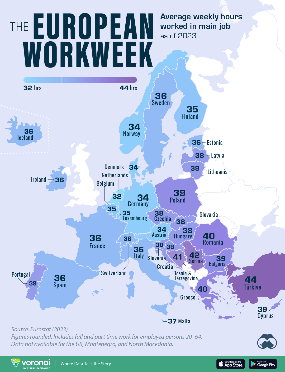
In Figure 1 (a), we have a choropleth map. What does choropleth¹ mean? And what kind of information could this map represent? The idea is to colour a specific area of the map, a district or state, based on a Quant or a Qual variable.

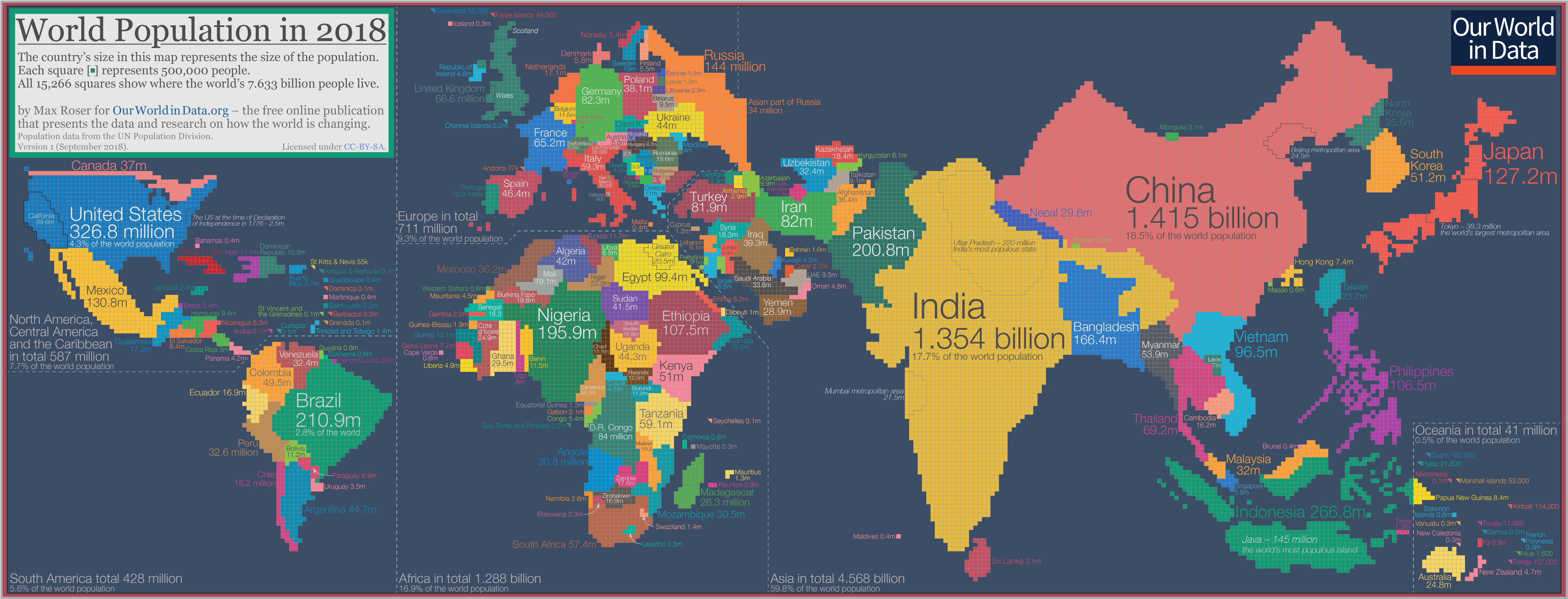
The Figure 1 (b) deliberately distorts and scales portions of the map in proportion to a Quant variable, in this case, population in 2018.

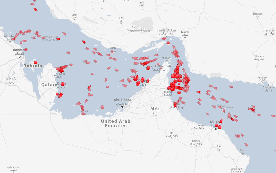
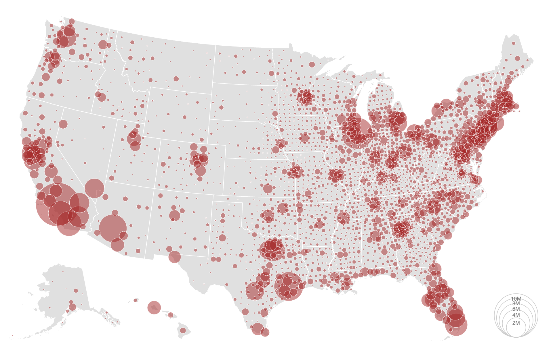
In Figure 2 (a) and Figure 2 (b), symbols are used to indicate either the location/presence of an item of interest, or a quantity by scaling their size in proportion to a Quant variable

Introduction

First; let us watch a short, noisy video on maps:

What kind of visualizations will we make?

Let us first understand the idea of a Geographical Information System, GIS:

We will first understand the structure of spatial data and where to find it. For now, we will deal with vector spatial data; the discussion on raster data will be dealt with in another future module.

We will get hands-on with making maps, both static and interactive.

Choropleth Map

Bubble Map

What information could this map below represent?

Let us now look at the slides. Then we will understand how the R packages sf, tmap work to create maps, using data downloadable into R using osmdata and osmplotr. We will also make interactive maps with leaflet and mapview; tmap is also capable of creating interactive maps.

View slides in full screen

Your Turn

Animal and Bird Migration

• Head off to movebank.org. Look at a few species of interest and choose one.
• Download the data ( ESRI Shapefile). Note: You will get a .zip file with a good many files in it. Save all of them, but read only the .shp file into R.
• Import that into R using sf_read()
• See how you can plot locations, tracks and colour by species….based on the data you download.
• For tutorial info: https://movebankworkshopraleighnc.netlify.app/

UFO Sightings

Here is a UFO Sighting dataset, containing location and text descriptions. https://github.com/planetsig/ufo-reports/blob/master/csv-data/ufo-scrubbed-geocoded-time-standardized.csv

Sales Data from kaggle

Head off to Kaggle and search for Geographical Sales related data. Make both static and interactive maps with this data. Justify your decisions for type of map.

References

1. Hadley Wickham, Danielle Navarro and Thomas Lin Pedersen. ggplot2: Elegant Graphics for Data Analysis, https://ggplot2-book.org/maps.html
2. Martijn Tennekes and Jakub Nowosad (2025). Elegant and informative maps with tmap. https://tmap.geocompx.org
3. Robin Lovelace, Jakub Nowosad, Jannes Muenchow. Geocomputation with R. https://r.geocompx.org/
   
4. Emine Fidan. Guide to Creating Interactive Maps in R, https://bookdown.org/eneminef/DRR_Bookdown/
   
5. Nikita Voevodin. R, Not the Best Practices, https://bookdown.org/voevodin_nv/R_Not_the_Best_Practices/maps.html
   
6. Want to make a cute logo-like map? Try https://prettymapp.streamlit.app
   
7. Free Map Tile services. https://alexurquhart.github.io/free-tiles/

R Package Citations

Package	Version	Citation
leaflet	2.2.2	Cheng et al. (2024)
osmdata	0.2.5	Mark Padgham et al. (2017)
rnaturalearth	1.0.1	Massicotte and South (2023)
sf	1.0.21	Pebesma (2018); Pebesma and Bivand (2023)
tmap	4.1	Tennekes (2018)

Cheng, Joe, Barret Schloerke, Bhaskar Karambelkar, and Yihui Xie. 2024. leaflet: Create Interactive Web Maps with the JavaScript “Leaflet” Library. https://doi.org/10.32614/CRAN.package.leaflet.

Mark Padgham, Bob Rudis, Robin Lovelace, and Maëlle Salmon. 2017. “Osmdata.” Journal of Open Source Software 2 (14): 305. https://doi.org/10.21105/joss.00305.

Massicotte, Philippe, and Andy South. 2023. rnaturalearth: World Map Data from Natural Earth. https://doi.org/10.32614/CRAN.package.rnaturalearth.

Pebesma, Edzer. 2018. “Simple Features for R: Standardized Support for Spatial Vector Data.” The R Journal 10 (1): 439–46. https://doi.org/10.32614/RJ-2018-009.

Pebesma, Edzer, and Roger Bivand. 2023. Spatial Data Science: With applications in R. Chapman and Hall/CRC. https://doi.org/10.1201/9780429459016.

Tennekes, Martijn. 2018. “tmap: Thematic Maps in R.” Journal of Statistical Software 84 (6): 1–39. https://doi.org/10.18637/jss.v084.i06.

Footnotes

1. Etymology. From Ancient Greek χώρα (khṓra, “location”) + πλῆθος (plêthos, “a great number”) + English map. First proposed in 1938 by American geographer John Kirtland Wright to mean “quantity in area,” although maps of the type have been used since the early 19th century.