The Grammar of Maps

Where is the Secret Garden?

Published

April 22, 2021

Modified

June 5, 2025

Abstract

Part of my Workshop course on R

Introduction

This RMarkdown document is part of my Workshop Course in R. The intent is to build Skill in coding in R, and also appreciate R as a way to metaphorically visualize information of various kinds, using predominantly geometric figures and structures.

All RMarkdown/Quarto files combine code, text, web-images, and figures developed using code. Everything is text; code chunks are enclosed in fences (```)

Goals

At the end of this Lab session, we should:
- know the types and structures of spatial data and be able to work with them
- understand the basics of modern spatial packages in R
- be able to specify and download spatial data from the web, using R from sources such as naturalearth and Open Streep Map
- plot static and interactive maps using ggplot, tmap and leaflet packages
- add symbols and markers for places and regions of our own interest in these maps.
- plot maps on a globe using the threejs package

Pedagogical Note

The method followed will be based on PRIMM:

PREDICT Inspect the code and guess at what the code might do, write predictions
RUN the code provided and check what happens
INFER what the parameters of the code do and write comments to explain. What bells and whistles can you see?
MODIFY the parameters code provided to understand the options available. Write comments to show what you have aimed for and achieved.
MAKE : take an idea/concept of your own, and graph it.

All jargon words will be capitalized and in bold font.

Set Up

The setup code chunk below brings into our coding session R packages that provide specific computational abilities and also datasets which we can use.

To reiterate: Packages and datasets are not the same thing !! Packages are (small) collections of programs. Datasets are just….information.

Setup the Packages

Run this in your Console first: devtools::install_github("ropensci/rnaturalearthhires")
Install all packages that are flagged by RStudio when you open this RMarkdown file

library(rnaturalearth)
library(rnaturalearthdata)

# Run this in your console first
# devtools::install_github("ropensci/rnaturalearthhires")
library(rnaturalearthhires)

# Plotting Maps
library(tidyverse) # Maps using ggplot + geom_sf
library(tmap) # Thematic Maps, static and interactive
library(tmaptools)
library(tmap.mapgl)
library(osmdata) # Fetch map data from osmdata.org
## Interactive Maps
library(leaflet) # interactive Maps
library(leaflet)
library(leaflet.providers)
library(leaflet.extras)
library(threejs) # Globe maps in R. Part of the htmlwidgets family of packages

# For Spatial Data Frame Processing
library(sf)

Introduction to Maps in R

We will take small steps in making maps using just two of the several map making packages in R.

The steps we will use are:

Search for an area of interest
Learn how to access spatial/map data using osmdata
Plot and dress up our map using ggplot and tmap
Create interactive maps with leaflet using a variety of map data providers. (Note: tmap can also do interactive maps which we will explore also.)

Bas. Onwards and Map-wards!!

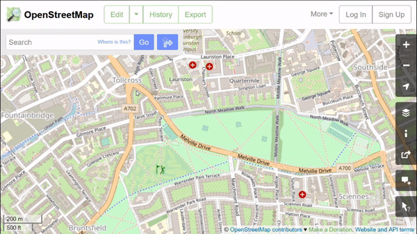
Step1 - Specifying an area of interest

In R, we need to specify a “BOUNDING BOX” first, to declare our area of interest. God made me a BengaluR-kaR…I think..Let’s see if we can declare an area of interest. Then we can order on Swiggy and…never mind.

We can declare a BOUNDING BOX in several ways.

Using a longitude latitude info from Bounding Box Tool which gives bounding boxes in many different formats.

Locate the place of interest using the search box.
click on the “box with arrow” tool on the upper left. This will create a rectangular shape.
Move/resize this box and then copy the bounding box from the menu at the bottom. Ensure you copy in CSV format.

# https://boundingbox.klokantech.com
# CSV: 77.574028,12.917262,77.595073,12.939895
bbox_1 <- matrix(
  c(77.574028, 12.917262, 77.595073, 12.939895),
  byrow = FALSE,
  nrow = 2,
  ncol = 2,
  dimnames = list(c("x", "y"), c("min", "max"))
)
bbox_1

       min      max
x 77.57403 77.59507
y 12.91726 12.93989

Using a place name to look up a BOUNDING BOX with osmdata::getbb. This may not always work if the place name is know well known.

# Using getbb command from the osmdata package
bbox_2 <- osmdata::getbb("Malleswaram, Bangalore, India")
bbox_2

       min      max
x 77.55033 77.59033
y 12.98274 13.02274

Let us examine both the calculated BOUNDING BOXes:

bbox_1

       min      max
x 77.57403 77.59507
y 12.91726 12.93989

bbox_2

       min      max
x 77.55033 77.59033
y 12.98274 13.02274

Both look similar in size; bbox_2 is slightly bigger.

We will use the bbox_2 from the above, to ensure we have a decent collection of features. If the download becomes too hefty, we can fall back on the smaller bbox!

Step2 - Get Map data

OpenStreetMap (OSM) provides maps of the world mostly created by volunteers. They are completely free to browse and use, with attribution to © OpenStreetMap contributors and adherence to the ODbL license required, and are used by many public and private organisations. OSM data can be downloaded in vector format and used for our own purposes. In this tutorial, we will obtain data from OSM using a query. A query is a request for data from a database. Simple queries can be performed more easily using the osmdata library for R, which automatically constructs the query and imports the data in a convenient format.

Open Street Map features have attributes in key-value pairs. We can use them to download the specific data we need. These features can easily be explored in the web browser, by using the ‘Query features’ button on OpenStreetMap (OSM):

Head off to OSM Street Map to try this out and to get an intuitive understanding of what OSM key-value pairs are, for different types of map features. Look for places of interest to you (features) and see what key-value pairs attach to those features.

NOTE: key-value pairs are also referred to as tags.

Useful key-value pairs / tags include:

KEY	VALUEs
building	yes (all), house residential, apartments
highway	residential, service, track, unclassified, footway, path
amenity	parking, parking_space, bench; place_of_worship; restaurant, cafe, fast_food; school, waste_basket, fuel, bank, toilets…
shop	convenience, supermarket, clothes, hairdresser, car-repair…
name	actual name of the place e.g. Main_Street, McDonald’s, Pizza Hut, Subway
waterway
natural
boundary

For more information see: OSM Tags for a nice visual description of popular key-value pairs that we can use. See what the highway tag looks like tag:highway

RapidEditor.Org for OSM Maps

For a user-friendly tutorial on how to edit and add features to the OSM map, head off to Rapid Editor. Here you will learn about OSM itself and about how you can add value to it by adding data from your own surroundings.

The osmdata commands available_features and available_tags can help also us get the associated key-value pairs to retrieve data from OSM.

osmdata::available_features() %>%
  as_tibble() %>%
  reactable::reactable(data = ., filterable = TRUE, minRows = 10)
available_tags(feature = "highway") %>% reactable::reactable(data = ., filterable = TRUE, minRows = 10)
available_tags(feature = "amenity") %>% reactable::reactable(data = ., filterable = TRUE, minRows = 10)
available_tags(feature = "natural") %>% reactable::reactable(data = ., filterable = TRUE, minRows = 10)

We can use these key-value pairs to download different types of map data. Within our bbox for Jayanagar, Bangalore, we want to download diverse kinds of FEATURE data. Remember that a FEATURE is any object that can be “seen” on a map. This is done using the OPQ query in the osmdata package. The main parameters for this command are:

bbox
KEY / VALUE pairs (“TAGS”) to specify the kind of feature you need

The query returns a list data structure, with all geometries and features within the bounding box, and we can use any or all of them. Now we know the map features we are interested in. We also know what key-value pairs will be used to get this info from OSM.

Data Downloads from OSM

Do not run these commands too many times. Re-run this ONLY if you have changed your BOUNDING BOX. We will get our map data from OSM and then save it avoid repeated downloads. So, please copy/paste and run the following commands in your console.

# This code is for reference
# Run these commands ONCE in your Console
# Or run this chunk manually one time

# Get all restaurants, atms, colleges within my bbox
locations <-
  osmdata::opq(bbox = bbox_2) %>%
  osmdata::add_osm_feature(
    key = "amenity",
    value = c("restaurant", "atm", "college")
  ) %>%
  osmdata_sf() %>% # Convert to Simple Features format
  purrr::pluck("osm_points") # Pull out the data frame of interest

# Get all buildings within my bbox
dat_buildings <-
  osmdata::opq(bbox = bbox_2) %>%
  osmdata::add_osm_feature(key = "building") %>%
  osmdata_sf() %>%
  purrr::pluck("osm_polygons")

# Get all residential roads within my bbox
dat_roads <-
  osmdata::opq(bbox = bbox_2) %>%
  osmdata::add_osm_feature(key = "highway") %>%
  osmdata_sf() %>%
  purrr::pluck("osm_lines")

# Get all parks / natural /greenery areas and spots within my bbox
dat_natural <-
  osmdata::opq(bbox = bbox_2) %>%
  osmdata::add_osm_feature(
    key = "natural",
    value = c("tree", "water", "wood")
  ) %>%
  osmdata_sf()
dat_natural

dat_trees <-
  dat_natural %>%
  purrr::pluck("osm_points")

dat_greenery <-
  dat_natural %>% pluck("osm_polygons")

Let us save this data, so we don’t need to download all this again! We will store the downloaded data as .gpkg files on our local hard drives to use when we run this file again later. We will name our stored files as buildings, roads, and greenery, and trees, each with the .gpkg file extension, e.g. trees.gpkg.

Check your local project folder for a subfolder titles /gpkg-data for these files after executing these commands.

# Eval is set to false here
# This code is for reference
# Run these commands ONCE in your Console
# Or manually run this chunk once

st_write(dat_roads,
  dsn = "./gpkg-data/roads.gpkg",
  append = FALSE, quiet = FALSE
)

st_write(dat_buildings,
  dsn = "./gpkg-data/buildings.gpkg",
  append = FALSE,
  quiet = FALSE
)

st_write(dat_greenery,
  dsn = "./gpkg-data/greenery.gpkg",
  append = FALSE, quiet = FALSE
)

st_write(dat_trees,
  dsn = "./gpkg-data/trees.gpkg",
  append = FALSE, quiet = FALSE
)

Work from here when you resume!

Always work from here to avoid repeated downloads from OSM. Start from the top ONLY if you intend to map new locations and need to modify your Bounding Box.

Let us now read back the saved Data:

buildings <- st_read("./gpkg-data/buildings.gpkg")

Reading layer `buildings' from data source 
  `/Users/arvindv/Documents/RWork/MyWebsites/my-quarto-website/content/labs/r-labs/maps/gpkg-data/buildings.gpkg' 
  using driver `GPKG'
Simple feature collection with 35007 features and 105 fields
Geometry type: POLYGON
Dimension:     XY
Bounding box:  xmin: 77.56221 ymin: 12.90906 xmax: 77.60373 ymax: 12.94971
Geodetic CRS:  WGS 84

greenery <- st_read("./gpkg-data/greenery.gpkg")

Reading layer `greenery' from data source 
  `/Users/arvindv/Documents/RWork/MyWebsites/my-quarto-website/content/labs/r-labs/maps/gpkg-data/greenery.gpkg' 
  using driver `GPKG'
Simple feature collection with 14 features and 10 fields
Geometry type: POLYGON
Dimension:     XY
Bounding box:  xmin: 77.57552 ymin: 12.91545 xmax: 77.60233 ymax: 12.94947
Geodetic CRS:  WGS 84

trees <- st_read("./gpkg-data/trees.gpkg")

Reading layer `trees' from data source 
  `/Users/arvindv/Documents/RWork/MyWebsites/my-quarto-website/content/labs/r-labs/maps/gpkg-data/trees.gpkg' 
  using driver `GPKG'
Simple feature collection with 797 features and 9 fields
Geometry type: POINT
Dimension:     XY
Bounding box:  xmin: 77.56566 ymin: 12.91545 xmax: 77.60233 ymax: 12.94947
Geodetic CRS:  WGS 84

roads <- st_read("./gpkg-data/roads.gpkg")

Reading layer `roads' from data source 
  `/Users/arvindv/Documents/RWork/MyWebsites/my-quarto-website/content/labs/r-labs/maps/gpkg-data/roads.gpkg' 
  using driver `GPKG'
Simple feature collection with 2662 features and 36 fields
Geometry type: LINESTRING
Dimension:     XY
Bounding box:  xmin: 77.55748 ymin: 12.90635 xmax: 77.60603 ymax: 12.95636
Geodetic CRS:  WGS 84

How many rows? ( Rows -> Features ) What kind of geom column in each data set?

# How many buildings?
nrow(buildings)

[1] 35007

buildings$geom

Geometry set for 35007 features 
Geometry type: POLYGON
Dimension:     XY
Bounding box:  xmin: 77.56221 ymin: 12.90906 xmax: 77.60373 ymax: 12.94971
Geodetic CRS:  WGS 84
First 5 geometries:

class(buildings$geom)

[1] "sfc_POLYGON" "sfc"

So the buildings dataset has 35007 buildings and their geometry is naturally a POLYGON type of geometry column.

Do this check for all the other spatial data, in the code chunk below. What kind of geom column does each dataset have?

My first Map in R

There are two ways of plotting maps that we will learn:

ggplot and geom_sf()

First we will plot with ggplot and geom_sf() : recall that our data is stored in 5 files: buildings, parks, roads, trees, and greenery.

ggplot() +
  geom_sf(
    data = buildings, fill = "gold", color = "grey",
    linewidth = 0.025
  ) + # POLYGONS
  geom_sf(data = roads, color = "#ff9999", linewidth = 0.5) + # LINES
  geom_sf(
    data = greenery, col = "darkseagreen",
    fill = "lightgreen",
    linewidth = 0.025
  ) + # POLYGONS
  geom_sf(data = trees, col = "darkgreen", size = 0.5) + # POINTS

  # Set plot limits to exactly the bbox_2
  # coord_sf(xlim = c(bbox_2[1,1], bbox_2[1,2]),
  #          ylim = c(bbox_2[2,1], bbox_2[2,2]),
  #          expand = FALSE) +
  theme_minimal()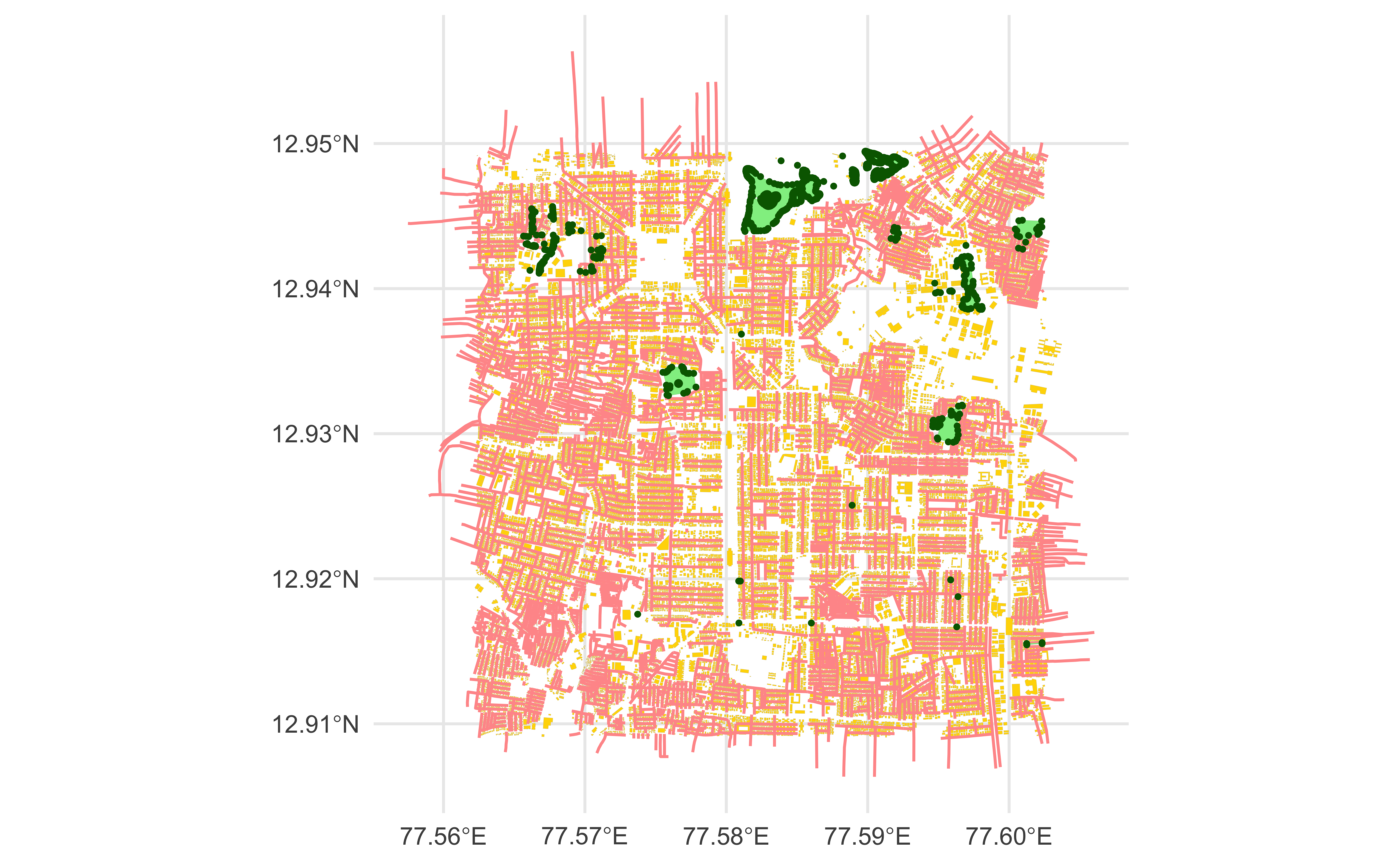

Note how geom_sf is capable of handling any geometry in the sfc column !!

geom_sf() is an unusual geom because it will draw different geometric objects depending on what simple features are present in the data: you can get points, lines, or polygons.

So there, we have our first map!

Map using `tmap` package

We can also create a map using a package called tmap. Here we also have the option of making the map interactive. tmap plots are made with code in “groups”: each group starts with a tm_shape() command.

## Let's see if we can Malleswaram look like Venice
## Red roof tops
# Group-1
tm_shape(buildings) +
  tm_polygons(fill = "firebrick", col = "firebrick") +

  # Group-2
  tm_shape(roads) +
  tm_lines(col = "black", lwd = 0.5) +

  # Group-3
  tm_shape(greenery) +
  tm_polygons(fill = "limegreen", col = "limegreen") +


  # Group-4
  # Malleswaram has only Banyan Trees, suppose
  tm_shape(trees) +
  tm_dots(fill = "darkgreen", size = 0.25)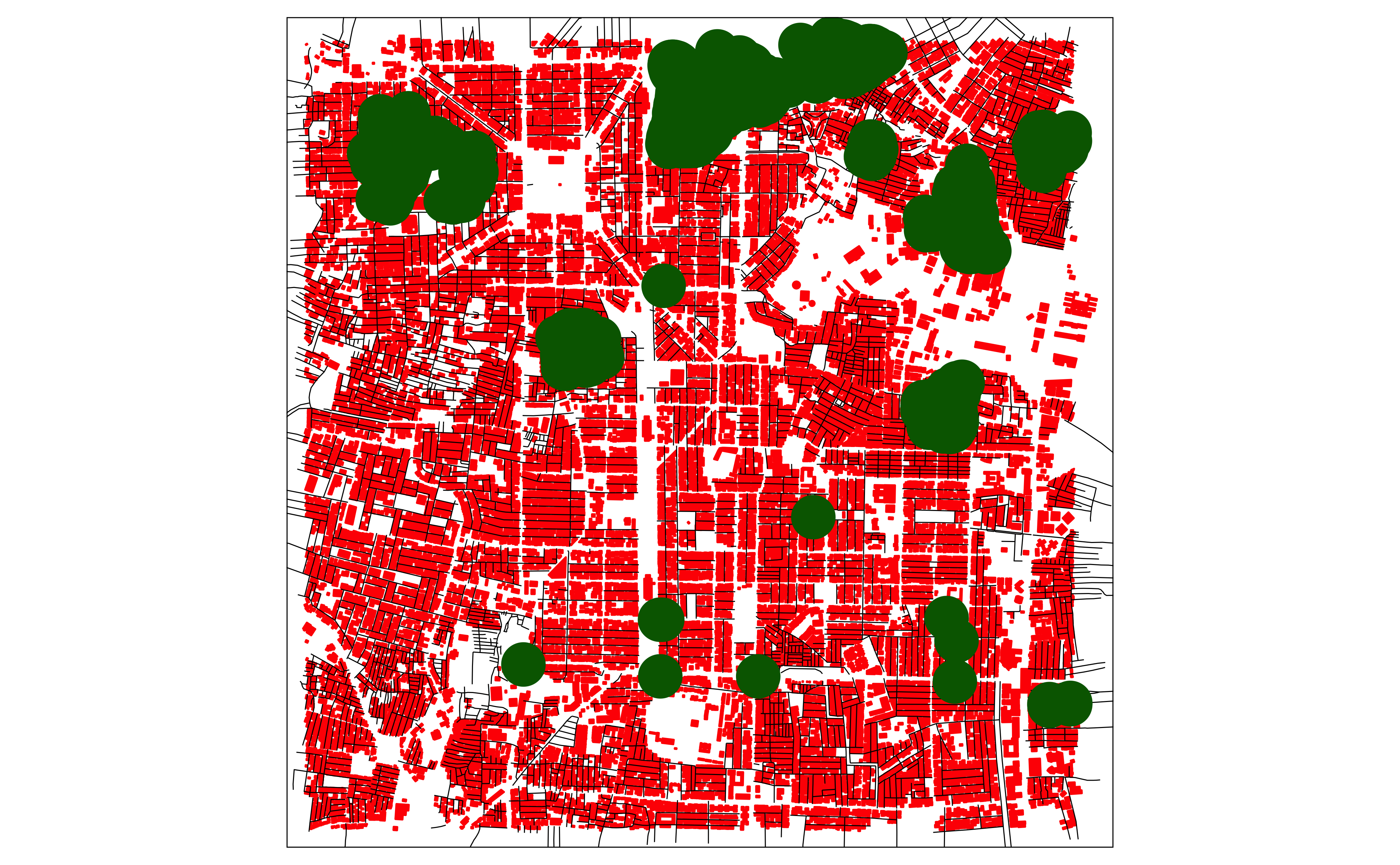

Using data from `tmap`

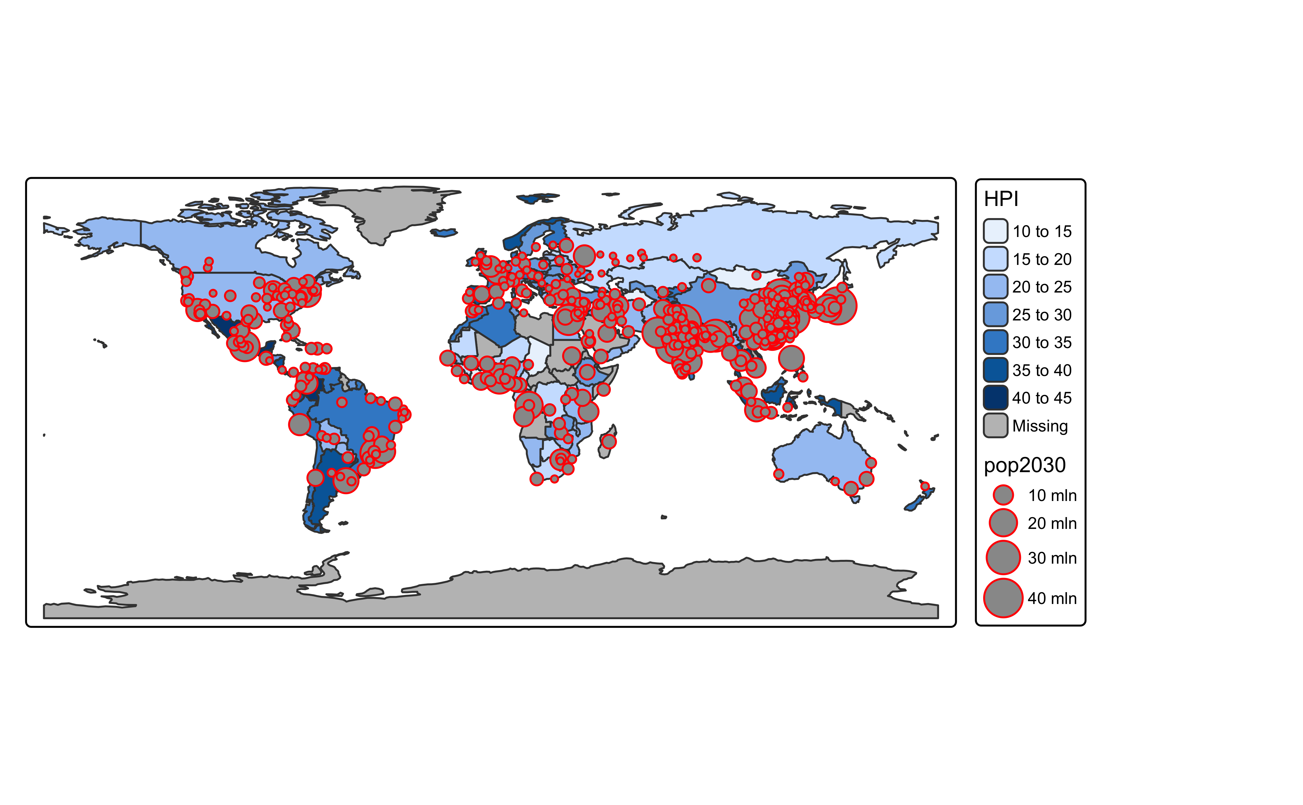
Like many other packages ( e.g. ggplot ) tmap also has a few built-in spatial datasets: World and metro, rivers, land and a few others. Check help on these. Let’s plot a first map using datasets built into tmap.

data("World")
head(World, n = 3)

ABCDEFGHIJ0123456789

	iso_a3 <fct>	name <fct>	sovereignt <fct>	continent <fct>	area <units>	pop_est <dbl>	pop_est_dens <dbl>	economy <fct>
1	AFG	Afghanistan	Afghanistan	Asia	652860 [km^2]	28400000	43.50090	7. Least developed region
2	AGO	Angola	Angola	Africa	1246700 [km^2]	12799293	10.26654	7. Least developed region
3	ALB	Albania	Albania	Europe	27400 [km^2]	3639453	132.82675	6. Developing region

We have several 14 attribute variables in World. Attribute variables such as gdp_cap_est, HPI are numeric. Others such as income_grp appear to be factors. iso_a3 is the standard three letter name for the country. name is of course, the name for each country!

data("metro")
head(metro, n = 3)

ABCDEFGHIJ0123456789

	name <chr>	name_long <chr>	iso_a3 <chr>	pop1950 <dbl>	pop1960 <dbl>	pop1970 <dbl>	pop1980 <dbl>	pop1990 <dbl>	pop2000 <dbl>
2	Kabul	Kabul	AFG	170784	285352	471891	977824	1549320	2401109
8	Algiers	El Djazair (Algiers)	DZA	516450	871636	1281127	1621442	1797068	2140577
13	Luanda	Luanda	AGO	138413	219427	459225	771349	1390240	2591388

Here too we have attribute variables for the metros, and they seem predominantly numeric. Again iso_a3 is the three letter name for the city.

tmap_mode("plot") # Making this a static plot

# Group 1
tm_shape(World) + # dataset = World.
  tm_polygons("HPI") + # Colour polygons by HPI numeric variable

  # Note the "+" sign continuation

  # Group 2
  tm_shape(metro) + # dataset = metro
  tm_bubbles(
    size = "pop2030",
    col = "red"
  ) +
  # Plot cities as bubbles
  # Size proportional to numeric variable `pop2030`

  tm_crs("auto")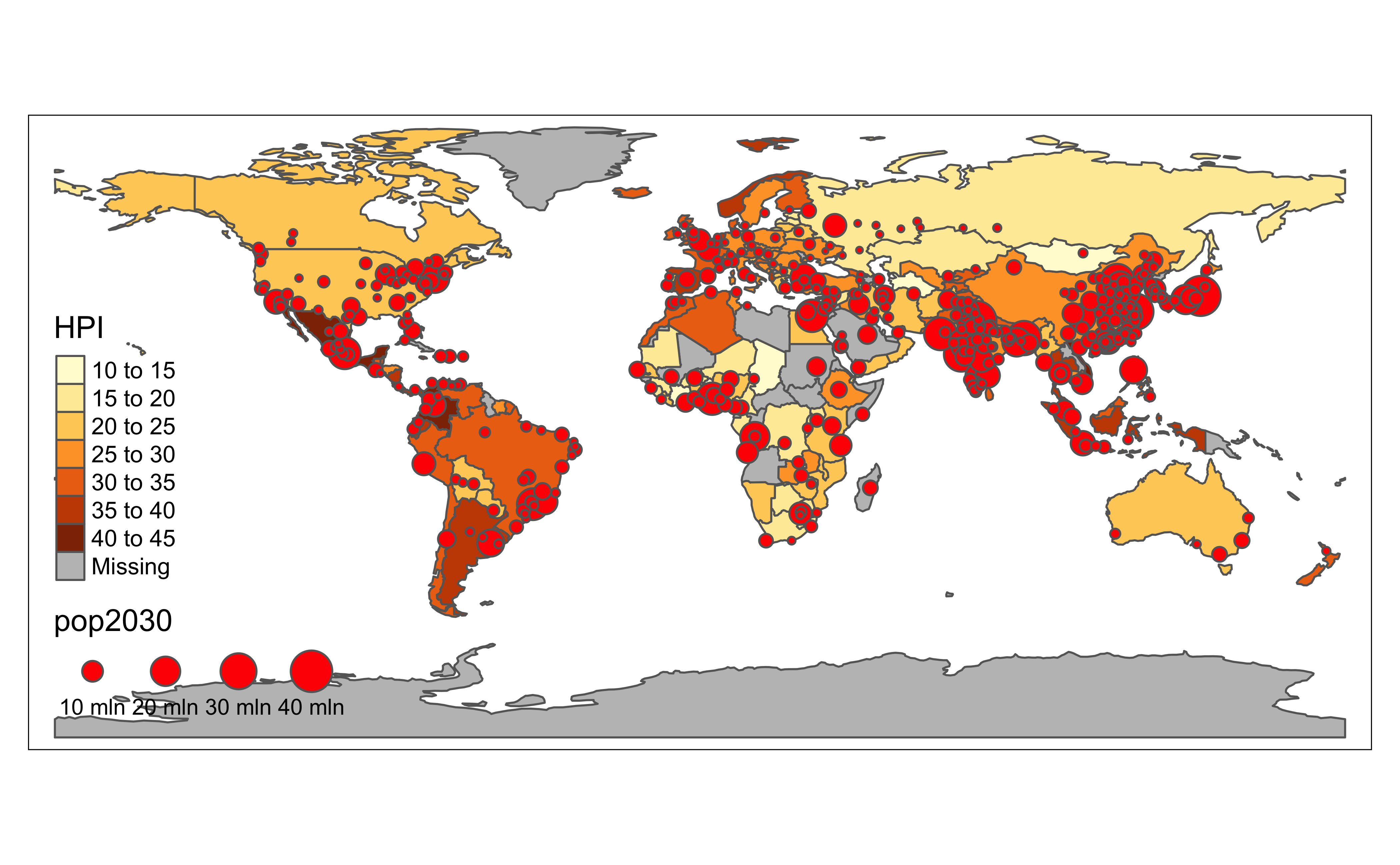

# tmap_mode("view")
# Let's use WaterColor Map this time!!
# tm_tiles("OpenTopoMap") +
tm_shape(World) +
  tm_polygons("HPI") + # Color by Happiness Index


  tm_shape(metro) +
  tm_bubbles(
    size = "pop2030", # Size City Markers by Population in 2020
    col = "red"
  )

Using data from `rnaturalearth`

The rnaturalearth package allows us to download shapes of countries. We can use it to get borders and also internal state/district boundaries.

india <-
  ne_states(
    country = "india",
    returnclass = "sf"
  ) # gives a ready sf dataframe !

india_neighbours <-
  ne_states(
    country = (c(
      "sri lanka", "pakistan",
      "afghanistan", "nepal", "bangladesh", "bhutan"
    )
    ),
    returnclass = "sf"
  )

Let’s look at the attribute variable columns to colour our graph and to shape our symbols:

names(india)

  [1] "featurecla" "scalerank"  "adm1_code"  "diss_me"    "iso_3166_2"
  [6] "wikipedia"  "iso_a2"     "adm0_sr"    "name"       "name_alt"  
 [11] "name_local" "type"       "type_en"    "code_local" "code_hasc" 
 [16] "note"       "hasc_maybe" "region"     "region_cod" "provnum_ne"
 [21] "gadm_level" "check_me"   "datarank"   "abbrev"     "postal"    
 [26] "area_sqkm"  "sameascity" "labelrank"  "name_len"   "mapcolor9" 
 [31] "mapcolor13" "fips"       "fips_alt"   "woe_id"     "woe_label" 
 [36] "woe_name"   "latitude"   "longitude"  "sov_a3"     "adm0_a3"   
 [41] "adm0_label" "admin"      "geonunit"   "gu_a3"      "gn_id"     
 [46] "gn_name"    "gns_id"     "gns_name"   "gn_level"   "gn_region" 
 [51] "gn_a1_code" "region_sub" "sub_code"   "gns_level"  "gns_lang"  
 [56] "gns_adm1"   "gns_region" "min_label"  "max_label"  "min_zoom"  
 [61] "wikidataid" "name_ar"    "name_bn"    "name_de"    "name_en"   
 [66] "name_es"    "name_fr"    "name_el"    "name_hi"    "name_hu"   
 [71] "name_id"    "name_it"    "name_ja"    "name_ko"    "name_nl"   
 [76] "name_pl"    "name_pt"    "name_ru"    "name_sv"    "name_tr"   
 [81] "name_vi"    "name_zh"    "ne_id"      "name_he"    "name_uk"   
 [86] "name_ur"    "name_fa"    "name_zht"   "FCLASS_ISO" "FCLASS_US" 
 [91] "FCLASS_FR"  "FCLASS_RU"  "FCLASS_ES"  "FCLASS_CN"  "FCLASS_TW" 
 [96] "FCLASS_IN"  "FCLASS_NP"  "FCLASS_PK"  "FCLASS_DE"  "FCLASS_GB" 
[101] "FCLASS_BR"  "FCLASS_IL"  "FCLASS_PS"  "FCLASS_SA"  "FCLASS_EG" 
[106] "FCLASS_MA"  "FCLASS_PT"  "FCLASS_AR"  "FCLASS_JP"  "FCLASS_KO" 
[111] "FCLASS_VN"  "FCLASS_TR"  "FCLASS_ID"  "FCLASS_PL"  "FCLASS_GR" 
[116] "FCLASS_IT"  "FCLASS_NL"  "FCLASS_SE"  "FCLASS_BD"  "FCLASS_UA" 
[121] "FCLASS_TLC" "geometry"

names(india_neighbours)

  [1] "featurecla" "scalerank"  "adm1_code"  "diss_me"    "iso_3166_2"
  [6] "wikipedia"  "iso_a2"     "adm0_sr"    "name"       "name_alt"  
 [11] "name_local" "type"       "type_en"    "code_local" "code_hasc" 
 [16] "note"       "hasc_maybe" "region"     "region_cod" "provnum_ne"
 [21] "gadm_level" "check_me"   "datarank"   "abbrev"     "postal"    
 [26] "area_sqkm"  "sameascity" "labelrank"  "name_len"   "mapcolor9" 
 [31] "mapcolor13" "fips"       "fips_alt"   "woe_id"     "woe_label" 
 [36] "woe_name"   "latitude"   "longitude"  "sov_a3"     "adm0_a3"   
 [41] "adm0_label" "admin"      "geonunit"   "gu_a3"      "gn_id"     
 [46] "gn_name"    "gns_id"     "gns_name"   "gn_level"   "gn_region" 
 [51] "gn_a1_code" "region_sub" "sub_code"   "gns_level"  "gns_lang"  
 [56] "gns_adm1"   "gns_region" "min_label"  "max_label"  "min_zoom"  
 [61] "wikidataid" "name_ar"    "name_bn"    "name_de"    "name_en"   
 [66] "name_es"    "name_fr"    "name_el"    "name_hi"    "name_hu"   
 [71] "name_id"    "name_it"    "name_ja"    "name_ko"    "name_nl"   
 [76] "name_pl"    "name_pt"    "name_ru"    "name_sv"    "name_tr"   
 [81] "name_vi"    "name_zh"    "ne_id"      "name_he"    "name_uk"   
 [86] "name_ur"    "name_fa"    "name_zht"   "FCLASS_ISO" "FCLASS_US" 
 [91] "FCLASS_FR"  "FCLASS_RU"  "FCLASS_ES"  "FCLASS_CN"  "FCLASS_TW" 
 [96] "FCLASS_IN"  "FCLASS_NP"  "FCLASS_PK"  "FCLASS_DE"  "FCLASS_GB" 
[101] "FCLASS_BR"  "FCLASS_IL"  "FCLASS_PS"  "FCLASS_SA"  "FCLASS_EG" 
[106] "FCLASS_MA"  "FCLASS_PT"  "FCLASS_AR"  "FCLASS_JP"  "FCLASS_KO" 
[111] "FCLASS_VN"  "FCLASS_TR"  "FCLASS_ID"  "FCLASS_PL"  "FCLASS_GR" 
[116] "FCLASS_IT"  "FCLASS_NL"  "FCLASS_SE"  "FCLASS_BD"  "FCLASS_UA" 
[121] "FCLASS_TLC" "geometry"

# Look only at attributes
india %>%
  st_drop_geometry() %>%
  head()

ABCDEFGHIJ0123456789

	featurecla <chr>	scalerank <int>	adm1_code <chr>	diss_me <int>	iso_3166_2 <chr>	wikipedia <chr>	iso_a2 <chr>	adm0_sr <int>
16	Admin-1 states provinces lakes	2	IND-20012	20012	IN-LA	NA	IN	1
43	Admin-1 states provinces lakes	2	IND-3299	3299	IN-AR	NA	IN	1
535	Admin-1 states provinces lakes	2	IND-3259	3259	IN-SK	NA	IN	1
538	Admin-1 states provinces lakes	2	IND-3257	3257	IN-WB	NA	IN	4
541	Admin-1 states provinces lakes	2	IND-2477	2477	IN-AS	NA	IN	1
695	Admin-1 states provinces lakes	2	IND-3254	3254	IN-UT	NA	IN	1

india_neighbours %>%
  st_drop_geometry() %>%
  head()

ABCDEFGHIJ0123456789

	featurecla <chr>	scalerank <int>	adm1_code <chr>	diss_me <int>	iso_3166_2 <chr>	wikipedia <chr>	iso_a2 <chr>	adm0_sr <int>	name <chr>
71	Admin-1 states provinces lakes	9	BTN-2484	2484	BT-TY	NA	BT	1	Tashi Yangtse
72	Admin-1 states provinces lakes	9	BTN-2483	2483	BT-44	NA	BT	1	Lhuntshi
73	Admin-1 states provinces lakes	9	BTN-2480	2480	BT-33	NA	BT	1	Bumthang
512	Admin-1 states provinces lakes	3	PAK-1111	1111	PK-GB	NA	PK	1	Northern Areas
536	Admin-1 states provinces lakes	9	BTN-2435	2435	BT-13	NA	BT	1	Ha
537	Admin-1 states provinces lakes	9	BTN-2438	2438	BT-14	NA	BT	1	Samchi

In the india data frame:

Column iso_a2 contains the country name.
Column name contains the name of the state

In the india_neighbours data frame:
- Column gu_a3 contains the country abbreviation
- Column name contains the name of the state
- Column iso_3166_2 contains the abbreviation of the state within each neighbouring country.

tmap_mode("plot")

# Plot India
tm_shape(india) +
  tm_polygons("name", # Colour by States in India
    fill.legend = tm_legend_hide()
  ) +

  # Plot Neighbours
  tm_shape(india_neighbours) +
  tm_fill(col = "gu_a3") + # Colour by Country Name

  # Plot the cities in India alone
  tm_shape(metro %>% dplyr::filter(iso_a3 == "IND")) +

  tm_dots(
    size = "pop2020",
    size.legend = tm_legend_hide()
  ) +
  # size by population in 2020

  tm_layout(legend.show = FALSE) +
  tm_credits("Geographical Boundaries are not accurate",
    size = 0.5,
    position = "right"
  ) +
  tm_compass(position = c("right", "top")) +
  tm_scalebar(position = "left") +
  tmap_style(style = "white")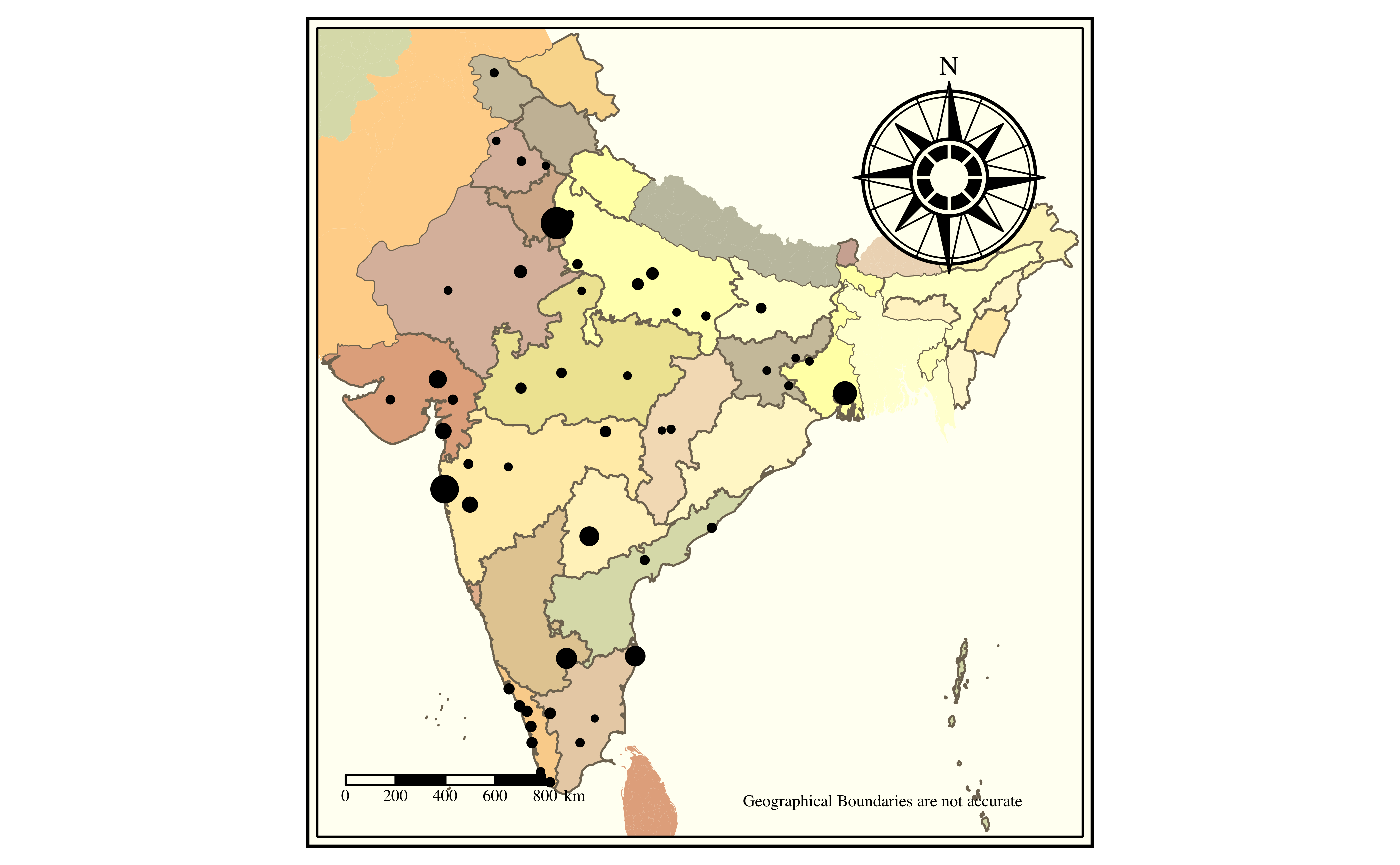

# Try other map styles
# cobalt #gray #white #watercolor #beaver #classic #watercolor #albatross #bw #col_blind

Your Turn 2

Can you try to download a map area of your home town and plot it as we have above?

Adding my favourite Restaurants to the map

Is it time to order on Swiggy…

Let us adding interesting places to our map: say based on your favourite restaurants etc. We need restaurant data: lat/long + name + maybe type of restaurant. This can be manually created ( like all of OSMdata ) or if it is already there we can download using key-value pairs in our OSM data query.

Restaurants can be downloaded using key= "amenity", value = "restaurant" or "cafe" etc. There are also other tags to explore!Searching for McDonalds for instance…( key = "name", value = "McDonalds"). Since we want JUST their location, and not the restaurant BUILDINGs, we extract osm_points.

# Again, run these commands in your Console
dat_R <-
  osmdata::opq(bbox = bbox_2) %>%
  osmdata::add_osm_feature(
    key = "amenity",
    value = c("restaurant")
  ) %>%
  osmdata_sf() %>%
  purrr::pluck("osm_points")

# Save the data for future use
write_sf(dat_R, dsn = "restaurants.gpkg", append = FALSE, quiet = FALSE)

Now reading the saved Restaurant Data:

restaurants <- st_read("./restaurants.gpkg")

Reading layer `restaurants' from data source 
  `/Users/arvindv/RWork/MyWebsites/my-quarto-website/content/labs/r-labs/maps/restaurants.gpkg' 
  using driver `GPKG'
Simple feature collection with 186 features and 63 fields
Geometry type: POINT
Dimension:     XY
Bounding box:  xmin: 77.55053 ymin: 12.98415 xmax: 77.5902 ymax: 13.02244
Geodetic CRS:  WGS 84

How many restaurants have we got?

restaurants %>% nrow()

[1] 225

So the restaurants dataset has 186 restaurants and their geometry is naturally a POINT type of geom column.

These are the names of columns in the Restaurant Data: Note the cuisine column.

glimpse(restaurants)

Rows: 225
Columns: 45
$ osm_id             <chr> "595408703", "595409635", "595409636", "595409790",…
$ name               <chr> "Ganesh Darshan", "Upahara Darshini", "Nagarjuna Ch…
$ addr.city          <chr> NA, NA, NA, NA, NA, NA, NA, NA, NA, NA, NA, NA, NA,…
$ addr.country       <chr> NA, NA, NA, NA, NA, NA, NA, NA, NA, NA, NA, NA, NA,…
$ addr.district      <chr> NA, NA, NA, NA, NA, NA, NA, NA, NA, NA, NA, NA, NA,…
$ addr.floor         <chr> NA, NA, NA, NA, NA, NA, NA, NA, NA, "0", NA, NA, NA…
$ addr.full          <chr> NA, NA, NA, NA, NA, NA, NA, NA, NA, NA, NA, NA, NA,…
$ addr.housename     <chr> NA, NA, NA, NA, NA, NA, NA, NA, NA, NA, NA, NA, NA,…
$ addr.housenumber   <chr> NA, NA, NA, NA, NA, NA, NA, "19/2", NA, NA, NA, NA,…
$ addr.postcode      <chr> NA, NA, NA, NA, NA, NA, NA, NA, NA, NA, NA, NA, NA,…
$ addr.street        <chr> NA, NA, NA, NA, NA, NA, NA, "South End Main Road", …
$ addr.suburb        <chr> NA, NA, NA, NA, NA, NA, NA, NA, NA, NA, NA, NA, NA,…
$ alt_name           <chr> NA, NA, NA, NA, NA, NA, NA, "Upahara Darshini", NA,…
$ amenity            <chr> "restaurant", "restaurant", "restaurant", "restaura…
$ brand              <chr> NA, NA, NA, NA, "Pizza Hut", NA, NA, NA, NA, NA, NA…
$ brand.wikidata     <chr> NA, NA, NA, NA, "Q191615", NA, NA, NA, NA, NA, NA, …
$ building           <chr> NA, NA, NA, NA, NA, NA, NA, NA, NA, NA, NA, NA, NA,…
$ capacity           <chr> NA, "150", NA, NA, NA, NA, NA, NA, NA, NA, NA, NA, …
$ check_date         <chr> NA, NA, NA, NA, NA, NA, NA, NA, NA, "2023-11-29", N…
$ cuisine            <chr> NA, NA, "indian", "italian", "pizza", NA, "indian",…
$ delivery           <chr> NA, NA, NA, NA, NA, NA, NA, NA, NA, NA, NA, NA, NA,…
$ description        <chr> NA, NA, NA, NA, NA, NA, NA, NA, NA, NA, NA, NA, NA,…
$ diet.vegetarian    <chr> NA, "only", NA, NA, NA, NA, NA, NA, NA, NA, NA, NA,…
$ email              <chr> NA, NA, NA, NA, NA, NA, NA, NA, NA, NA, NA, NA, NA,…
$ internet_access    <chr> NA, NA, NA, NA, NA, NA, NA, NA, NA, NA, NA, NA, NA,…
$ level              <chr> NA, NA, NA, NA, NA, NA, NA, NA, NA, "0", NA, NA, NA…
$ name.en            <chr> NA, NA, NA, NA, NA, NA, NA, NA, NA, NA, NA, NA, NA,…
$ name.kn            <chr> "ಗಣೇಶ ದರ್ಶಿನಿ", "ಉಪಹಾರ ದರ್ಶಿನಿ", "ನಾಗಾರ್ಜುನ ಚಿಮಿನಿ", "ಲಾ ಕಾಸಾ…
$ note               <chr> NA, NA, NA, NA, NA, NA, NA, NA, NA, NA, NA, NA, NA,…
$ opening_hours      <chr> NA, NA, NA, NA, NA, NA, NA, NA, NA, NA, NA, NA, NA,…
$ operator           <chr> NA, NA, NA, NA, NA, NA, NA, NA, NA, NA, NA, NA, NA,…
$ outdoor_seating    <chr> NA, NA, NA, NA, NA, NA, NA, NA, NA, NA, NA, NA, NA,…
$ payment.mastercard <chr> NA, NA, NA, NA, NA, NA, NA, NA, NA, NA, NA, NA, NA,…
$ payment.visa       <chr> NA, NA, NA, NA, NA, NA, NA, NA, NA, NA, NA, NA, NA,…
$ phone              <chr> NA, NA, NA, NA, NA, NA, NA, NA, NA, NA, NA, NA, NA,…
$ smoking            <chr> NA, NA, NA, NA, NA, NA, NA, NA, NA, NA, NA, NA, NA,…
$ source             <chr> NA, NA, NA, NA, NA, NA, NA, NA, NA, NA, NA, NA, NA,…
$ survey.date        <chr> NA, NA, NA, NA, NA, NA, NA, NA, NA, NA, NA, NA, NA,…
$ takeaway           <chr> NA, "yes", NA, NA, NA, NA, NA, NA, NA, NA, NA, NA, …
$ toilets.wheelchair <chr> NA, NA, NA, NA, NA, NA, NA, NA, NA, NA, NA, NA, "no…
$ website            <chr> NA, NA, NA, NA, NA, NA, NA, NA, NA, NA, NA, NA, NA,…
$ wheelchair         <chr> NA, NA, NA, NA, NA, "no", NA, NA, NA, NA, NA, "no",…
$ wikidata           <chr> NA, NA, NA, NA, NA, NA, NA, NA, NA, NA, NA, NA, NA,…
$ wikipedia          <chr> NA, NA, NA, NA, NA, NA, NA, NA, NA, NA, NA, NA, NA,…
$ geom               <POINT [°]> POINT (77.58403 12.93092), POINT (77.58442 12…

So let us plot the restaurants as POINTs using the restaurants data we have downloaded. The cuisine attribute looks interesting; let us colour the POINT based on the cuisine offered at that restaurant.

So Let’s look therefore at the cuisine column!

# ( I want pizza...)
restaurants$cuisine %>% unique()

 [1] NA                                             
 [2] "indian"                                       
 [3] "italian"                                      
 [4] "pizza"                                        
 [5] "regional"                                     
 [6] "ice_cream"                                    
 [7] "chinese"                                      
 [8] "american"                                     
 [9] "South_Indian"                                 
[10] "Multi-cuisne"                                 
[11] "South_India"                                  
[12] "chicken;regional"                             
[13] "arab"                                         
[14] "indian;seafood;fine_dining"                   
[15] "fast_food"                                    
[16] "kebab;grill"                                  
[17] "chicken"                                      
[18] "chinese;sandwich;tea;indian;coffee_shop"      
[19] "indian,_japanese"                             
[20] "indian;regional"                              
[21] "asian"                                        
[22] "indian;seafood"                               
[23] "south_indian"                                 
[24] "indian;chinese;tibetan;regional;kebab;chicken"

Big mess…many NAs, some double entries, separated by commas and semicolons….

The cuisine attribute:

Note: The cuisine variable has more than one entry for a given restaurant. We use tidyr::separate_*_*() to make multiple columns out of the cuisine column and retain the first one only. Since the entries are badly entered using both “;” and “,” we need to do this twice ;-() Bad Data entry!!

Let’s get one cuisine entry per restaurant, and drop off the ones that do not mention a cuisine at all:

restaurants <- restaurants %>%
  drop_na(cuisine) %>% # Knock off nondescript restaurants

  # Some have more than one classification ;-()
  # Separated by semicolon or comma, so....
  separate_wider_delim(
    cols = cuisine,
    names = c("cuisine", NA, NA),
    delim = ";",
    too_few = "align_start",
    too_many = "drop"
  ) %>%
  separate_wider_delim(
    cols = cuisine,
    names = c("cuisine", NA, NA),
    delim = ",",
    too_few = "align_start",
    too_many = "drop"
  )

# Finally good food?
restaurants$cuisine

  [1] "indian"       "indian"       "chinese"      "indian"       "indian"      
  [6] "indian"       "indian"       "regional"     "regional"     "indian"      
 [11] "regional"     "regional"     "indian"       "chicken"      "italian"     
 [16] "chinese"      "regional"     "indian"       "japanese"     "regional"    
 [21] "indian"       "regional"     "seafood"      "Bengali"      "regional"    
 [26] "chats"        "regional"     "regional"     "indian"       "indian"      
 [31] "indian"       "fast_food"    "fast_food"    "indian"       "indian"      
 [36] "indian"       "fast_food"    "indian"       "regional"     "chinese"     
 [41] "indian"       "chinese"      "regional"     "regional"     "regional"    
 [46] "regional"     "regional"     "regional"     "regional"     "pizza"       
 [51] "regional"     "regional"     "regional"     "regional"     "regional"    
 [56] "regional"     "regional"     "regional"     "regional"     "regional"    
 [61] "indian"       "regional"     "regional"     "regional"     "regional"    
 [66] "regional"     "indian"       "indian"       "indian"       "regional"    
 [71] "regional"     "indian"       "regional"     "indian"       "regional"    
 [76] "regional"     "pizza"        "regional"     "regional"     "regional"    
 [81] "regional"     "regional"     "asian"        "persian"      "american"    
 [86] "regional"     "regional"     "regional"     "regional"     "regional"    
 [91] "french"       "tex-mex"      "indian"       "pizza"        "asian"       
 [96] "punjabi"      "south_indian" "indian"       "mexican"      "regional"

Looks clean! Each entry is only ONE and not multiple any more. Now let’s plot the Restaurants as POINTs:

# http://www.stat.columbia.edu/~tzheng/files/Rcolor.pdf
#
ggplot() +
  geom_sf(data = buildings, colour = "firebrick") +
  geom_sf(data = roads, colour = "gold", linewidth = 0.25) +
  geom_sf(
    data = restaurants %>% drop_na(cuisine),
    aes(fill = cuisine, geometry = geom),
    colour = "black",
    shape = 21,
    size = 3
  ) +
  # Set plot limits to exactly the bbox_2
  # coord_sf(xlim = c(bbox_2[1,1], bbox_2[1,2]),
  #          ylim = c(bbox_2[2,1], bbox_2[2,2]),
  #          expand = FALSE) +
  theme_minimal() +
  theme(legend.position = "right") +
  labs(
    title = "Restaurants in Malleswaram, Bangalore",
    caption = "Based on osmdata"
  )

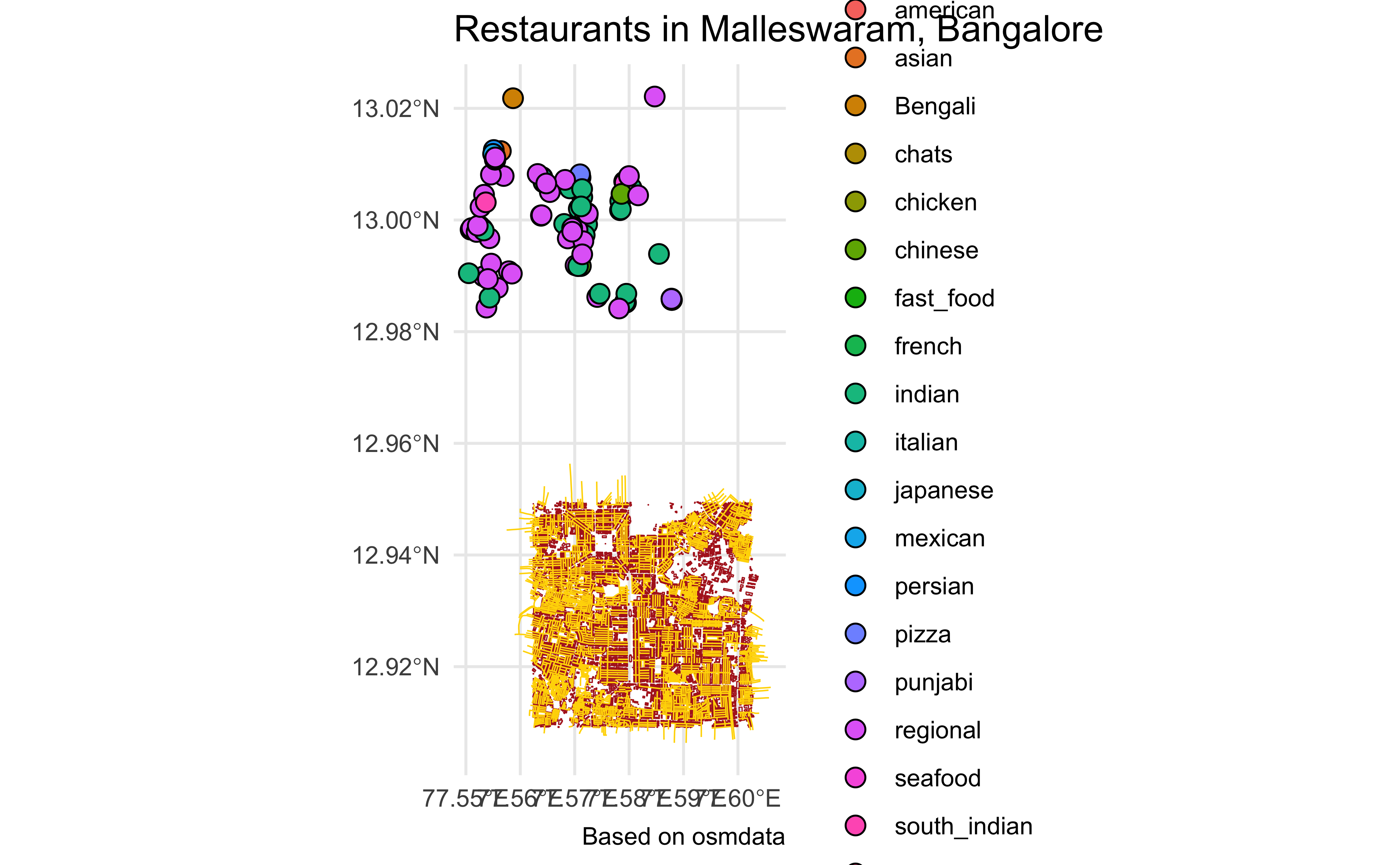
We could have done a (much!) better job, by combining cuisines into simpler and fewer categories, ( South_India and South_Indian ), but that is for another day!!

By now we know that we can use geom_sf() multiple number of times with different datasets to create layered maps in R.

Some fancy stuff

Let us try making glob based maps with the package threejs. This package is one of the family of packages in the htmlwidgets group of packages. It allows the use of some ( famous!) JavaScript graphing libraries directly and natively in R.

`globejs` usage

The globejs command from the package threejs allows one to plot points, arcs and images on a globe in 3D. The globe can be rotated and and zoomed. Great Circles and historical routes are a good idea for this perhaps.

Refer to this page for more ideas http://bwlewis.github.io/rthreejs/globejs.html

We will generate some random locations and plot them on the 3D globe.

# Random Lats and Longs
lat <- rpois(10, 60) + rnorm(10, 80)
long <- rpois(10, 60) + rnorm(10, 10)

# Random "Spike" heights for each location. Population? Tourists? GDP?
value <- rpois(10, lambda = 80)

globejs(lat = lat, long = long)

As seen, “spikes” are created at the random lat-lon locations. We can control the height/width/colour of the spikes, as well as the initial view of the globe itself: zoom, location and so on

globejs(
  lat = lat,
  long = long,

  # random heights of the Spikes (!!) at lat-long combo
  value = value,
  color = "red",
  # Zoom factor, default is 35
  fov = 50
)

globejs(
  lat = lat,
  long = long,
  value = value,
  color = "red",
  pointsize = 4, # width of the columns
  # Zoom position
  fov = 35,
  # initial position of the globe
  rotationlat = 0.6, #  in RADIANS !!! Good Heavens!!
  rotationlong = 0.2 #  in RADIANS !!! Good Heavens!!
)

globejs(
  lat = lat,
  long = long,
  value = value,
  color = "red",
  pointsize = 4,
  fov = 35,
  rotationlat = 0.6,
  rotationlong = 0.2,
  lightcolor = "#aaeeff",
  emissive = "#0000ee",
  bodycolor = "#ffffff",
  bg = "grey"
)

Scope and Packages for Exploration!!

sfnetworks / tmap networks

mapsf

ggspatial

Resources

Free Map Tile services. https://alexurquhart.github.io/free-tiles/
Martijn Tennekes and Jakub Nowosad (2025). Elegant and informative maps with tmap. https://tmap.geocompx.org
Emine Fidan, Guide to Creating Interactive Maps in R
Nikita Voevodin,R, Not the Best Practices
RapidEditor.Org. Web-based editor for community-data addition to OSM Maps. Can be used to really add value to local mappers and for your own projects.

Assignments

Draw a map of your home-town with your favourite restaurants shown. Pop-ups for each restaurant will win bonus points.
Download bird migration data from movebank.org. Import these into R and plot a migration map using tmap. Include the graticule, compass, legend, and credits.

Inspiration

Burkhart, Christian. n.d. “Streetmaps.” StreetMaps

Making Vector Maps, Computing for the Social Sciences, Univ. of Chicago

Introduction

Goals

Pedagogical Note

Set Up

Setup the Packages

Introduction to Maps in R

Step1 - Specifying an area of interest

Step2 - Get Map data

My first Map in R

ggplot and geom_sf()

Map using tmap package

Using data from tmap

Using data from rnaturalearth

Your Turn 2

Adding my favourite Restaurants to the map

Some fancy stuff

globejs usage

Scope and Packages for Exploration!!

sfnetworks / tmap networks

mapsf

ggspatial

Resources

Assignments

Inspiration

Map using `tmap` package

Using data from `tmap`

Using data from `rnaturalearth`

`globejs` usage