library(tidyverse)
library(sf)
##
# Mapview and allied packages
library(mapview)
library(leaflet)
library(leafem) # Provides extensions for packages 'leaflet' & 'mapdeck', many of which are used by package 'mapview'.
library(leafgl) # High-Performance 'WebGl' Rendering for Package 'leaflet'
library(leafsync) # Create small multiples of several leaflet web maps with (optional) synchronised panning and zooming control.
##
library(slideview) # Create a side-by-side view of raster(image)s with an interactive slider to switch between regions of the images.
library(cubeview) # View 3D Raster Cubes Interactively
library(plainview) # Provides methods for plotting potentially large (raster) images interactively on a plain HTML canvas.
# Data
library(osmdata) # Import OSM Vector Data into R
# library(osmplotr) # Creating maps with OSM data in R. Package is no longer maintained, so not used.Playing With Mapview
Abstract
Making Interactive maps in R, using the mapview package
Keywords
maps, mapview, interactive
Introduction
In this tutorial, we will learn to create interactive maps in R, using a package called mapview, which is a simpler way to access leaflet, which is a wellknown package to create interactive maps.
Leaflet is a JavaScript library for creating dynamic maps that support panning and zooming along with various annotations like markers, polygons, and popups.
Whereas leaflets code becomes lengthy fairly quickly, mapview allows full functionality of leaflet using sensible defaults. Type ?mapview in the console for more help.
More Information
More information on mapview is available at https://r-spatial.github.io/mapview/.
There are also two wonderful talks by Tim Appelhans, the creator of mapview that are available here:
Basic Maps using mapview
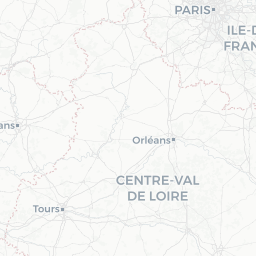
franconia , trails, and breweries are geospatial datasets of class sf from the mapview package. franconia contains MULTIPOLYGON, trails contains MULTILINESTRING, and breweries contains POINT geometries.
class(franconia)[1] "sf" "data.frame"head(franconia, 1)NUTS_ID <chr> | SHAPE_AREA <dbl> | SHAPE_LEN <dbl> | CNTR_CODE <fct> | NAME_ASCI <fct> | geometry <s_MULTIP> | district <chr> | |
|---|---|---|---|---|---|---|---|
| 1 | DE241 | 0.006736012 | 0.3926225 | DE | Bamberg, Kreisfreie Stadt | <s_MULTIP> | Oberfranken |
class(trails)[1] "sf" "data.frame"head(trails, 1)FGN <chr> | FKN <fct> | district <chr> | geometry <s_MULTIL> | |
|---|---|---|---|---|
| 1 | 003756/Kunigundenweg | 003756 | Oberfranken | <s_MULTIL> |
class(breweries)[1] "sf" "data.frame"head(breweries, 1)brewery <chr> | address <chr> | zipcode <chr> | village <chr> | state <fct> | founded <dbl> | number.of.types <dbl> | number.seasonal.beers <dbl> | geometry <sf_POINT> | |
|---|---|---|---|---|---|---|---|---|---|
| 1 | Brauerei Rittmayer | Aischer Hauptstrasse 5 | 91325 | Adelsdorf | Bayern | 1422 | 2 | 1 | <sf_POINT> |
Plotting these is a simple one-liner:


mapview has automagically added shapes to the map by detecting the geometry column in each sf dataframe. (rather like geom_sf in ggplot). The map is interactive and clicking on any of the shapes provides a popup containing all the remaining attribute information ( from the non-geometry columns)
Note that there are multiple basemaps available by default in mapview. The layers icon on the left allows the user to interactively choose the base map style. There are other basemaps that can be specified programmatically.
We can also plot these maps as overlays ( since they all pertain to the same geographical area.) Each of the maps can also be given a layer name:
# Single overlay plot with layer names
mapview(franconia, layer.name = "1-Franconia") +
mapview(trails, layer.name = "2-Brewery Trails") +
mapview(breweries, layer.name = "3-Breweries")


Add Colours to Shapes
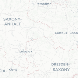
mapview offers a simple way of adding colours to shapes, based on any of the other columns in the respective dataframe, by passing that column name(in quotes!) to the parameter zcol in mapview():
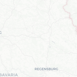
mapview(franconia,
zcol = "district",
col.regions = grDevices::hcl.colors
) + # set colour palette
mapview(breweries, col.regions = "red")franconia - district
MittelfrankenOberfranken
Unterfranken
breweries
50 km
30 mi
Legends
Note that legends are created by default. They can be turned off with ,legend = FALSE inside the mapview() function. Note also the home button at the bottom right: that re-centres and resets the map.
Map Stack with All Attributes
One can get a stack of maps where the shapes are coloured by all variables simultaneously by using , burst = TRUE instead of zcol:
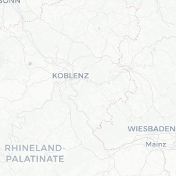
mapview(franconia, burst = TRUE)NUTS_ID
DE241DE242
DE243
DE244
DE245
DE246
DE247
DE248
DE249
DE24A
DE24B
DE24C
DE24D
DE251
DE252
DE253
DE254
DE255
DE256
DE257
DE258
DE259
DE25A
DE25B
DE25C
DE261
DE262
DE263
DE264
DE265
DE266
DE267
DE268
DE269
DE26A
DE26B
DE26C
SHAPE_AREA
SHAPE_LEN
CNTR_CODE
DENAME_ASCI
Ansbach, Kreisfreie StadtAnsbach, Landkreis
Aschaffenburg, Kreisfreie Stadt
Aschaffenburg, Landkreis
Bad Kissingen
Bamberg, Kreisfreie Stadt
Bamberg, Landkreis
Bayreuth, Kreisfreie Stadt
Bayreuth, Landkreis
Coburg, Kreisfreie Stadt
Coburg, Landkreis
Erlangen-Hochstadt
Erlangen, Kreisfreie Stadt
Forchheim
Furth, Kreisfreie Stadt
Furth, Landkreis
Hassberge
Hof, Kreisfreie Stadt
Hof, Landkreis
Kitzingen
Kronach
Kulmbach
Lichtenfels
Main-Spessart
Miltenberg
Neustadt a. d. Aisch-Bad Windsheim
Nurnberger Land
Nurnberg, Kreisfreie Stadt
Rhon-Grabfeld
Roth
Schwabach, Kreisfreie Stadt
Schweinfurt, Kreisfreie Stadt
Schweinfurt, Landkreis
Weissenburg-Gunzenhausen
Wunsiedel i. Fichtelgebirge
Wurzburg, Kreisfreie Stadt
Wurzburg, Landkreis
district
MittelfrankenOberfranken
Unterfranken
50 km
30 mi
Using mapview with external geospatial data
On to something more complex. We want to plot a known set of locations on a mapview map. mapview takes in geographical data in many ways and we will explore most of them.
Data Sources for mapview
Objects of the following spatial classes are supported in
mapview:
Which means we cannot give mapview simple vectors / matrices/ dataframes containing lon / lat information: they need to be converted into sf format first. (Leaflet could natively do this! Hmm…)
Let us read in the data set from data.world that gives us POINT locations of all airports in India in a data frame / tibble. The dataset is available at India Airports Locations.
You can either download it, save a copy, and read it in as usual, or use the URL itself to read it in directly from data.world. In the latter case, you will need the package data.world and also need to register your credentials for that page with RStudio. The (very simple!) instructions are available here at data.world
# library(devtools)
# devtools::install_github("datadotworld/data.world-r", build_vignettes = TRUE)
library(data.world)
india_airports <-
read_csv(file = "https://query.data.world/s/ahtyvnm2ybylf65syp4rsb5tulxe6a") %>%
slice(-1) %>% # Drop the first row which contains labels
dplyr::mutate(
id = as.integer(id),
latitude_deg = as.numeric(latitude_deg),
longitude_deg = as.numeric(longitude_deg),
elevation_ft = as.integer(elevation_ft)
) %>%
rename("lon" = longitude_deg, "lat" = latitude_deg) %>%
# Remove four locations which seem to be in the African Atlantic
filter(!id %in% c(330834, 330867, 325010, 331083)) %>%
# Convert to `sf` dataframe
st_as_sf(
coords = c("lon", "lat"),
remove = FALSE, # retain the original lon and lat columns
sf_column_name = "geometry",
crs = 4326 # specify Projection,else no basemap will be plotted
)
india_airports %>% head()id <int> | ident <chr> | type <chr> | name <chr> | lat <dbl> | lon <dbl> | elevation_ft <int> | continent <chr> | iso_country <chr> | iso_region <chr> | |
|---|---|---|---|---|---|---|---|---|---|---|
| 26555 | VIDP | large_airport | Indira Gandhi International Airport | 28.56650 | 77.1031 | 777 | AS | IN | IN-DL | |
| 26434 | VABB | large_airport | Chhatrapati Shivaji International Airport | 19.08870 | 72.8679 | 39 | AS | IN | IN-MM | |
| 35145 | VOBL | large_airport | Kempegowda International Airport | 13.19790 | 77.7063 | 3000 | AS | IN | IN-KA | |
| 26618 | VOMM | large_airport | Chennai International Airport | 12.99001 | 80.1693 | 52 | AS | IN | IN-TN | |
| 26444 | VAGO | large_airport | Dabolim Airport | 15.38080 | 73.8314 | 150 | AS | IN | IN-GA | |
| 26609 | VOCI | large_airport | Cochin International Airport | 10.15200 | 76.4019 | 30 | AS | IN | IN-KL |
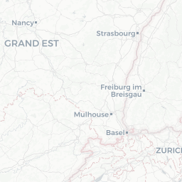
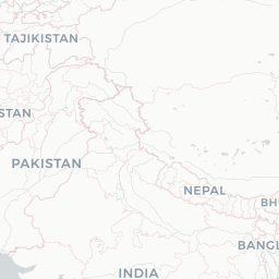
Let us plot this in `mapview`, using an ESRI National Geographic style map instead of the OSM Base Map. We will also place small circle markers for each airport.
# Change the order of basemaps in mapview
# Male OpenTopoMap the default
mapviewOptions(basemaps = c("OpenTopoMap", "CartoDB.Positron", "CartoDB.DarkMatter", "OpenStreetMap", "Esri.WorldImagery"))
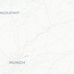
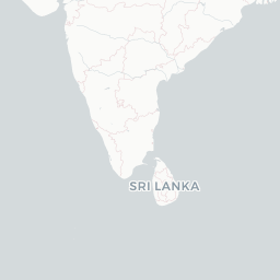
mapview(india_airports,
zcol = "type"
)


india_airports - type
closedheliport
large_airport
medium_airport
small_airport
500 km
500 mi
Using popups and labels
By default, mapview provides a mouseover label information (feature ID, or a zcol attribute if zcol has been set), and a popup table containing all attribute fields. This can be customized to show the user wants. There are various options for popups in mapview:
popup = popupTable()Text/table based popuppopup = popupImage()Images in popupspopup = popupGraph()a data visualization in the popup-
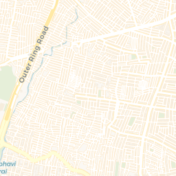
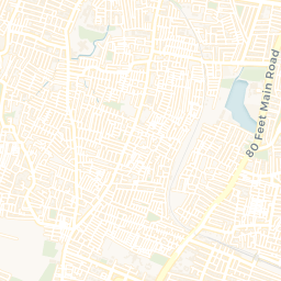
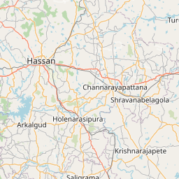
popup = popupIframe()URL, Image, Video in a popup using iframeWe will download a small dataset of restaurants in say Malleswaram, Bangalore and plot them with
mapview, adding popups and labels:
# library(osmdata)
bbox <- osmdata::getbb("Malleswaram, Bengaluru")
bbox min max
x 77.55033 77.59033
y 12.98274 13.02274restaurants <-
osmdata::opq(bbox = bbox) %>%
osmdata::add_osm_feature(
key = "amenity",
value = "restaurant"
) %>%
osmdata_sf() %>% # Convert to Simple Features format
purrr::pluck("osm_points") # Pull out the data frame of interest
restaurants <- restaurants %>%
dplyr::filter(cuisine == "indian")
restaurantsosm_id <chr> | name <chr> | addr:city <chr> | addr:country <chr> | addr:district <chr> | addr:floor <chr> | addr:full <chr> | addr:hamlet <chr> | ||
|---|---|---|---|---|---|---|---|---|---|
| 461539222 | 461539222 | Adiga's | NA | NA | NA | NA | NA | NA | |
| 598500940 | 598500940 | Udupi Sri Krishnarajathadri | NA | NA | NA | NA | NA | NA | |
| 673377213 | 673377213 | Sana Di Ge | NA | NA | NA | NA | NA | NA | |
| 673860152 | 673860152 | New Shanthi Sagar | NA | NA | NA | NA | NA | NA | |
| 1116484556 | 1116484556 | Kabab Studio | NA | NA | NA | NA | NA | NA | |
| 1448082496 | 1448082496 | Sai Shakti | NA | NA | NA | NA | NA | NA | |
| 2025970848 | 2025970848 | Coastal Express | NA | NA | NA | NA | NA | NA | |
| 2303827881 | 2303827881 | Sattvam | NA | NA | NA | NA | NA | NA | |
| 2631196051 | 2631196051 | Maiyas | NA | NA | NA | NA | NA | NA | |
| 4008859835 | 4008859835 | Shristi Sagar | Bangalore | NA | NA | NA | NA | NA |
Let us add popups containing the restaurant name and cuisine; we need to add the R package leafpop to add popups
library(leafpop)
mapviewOptions(basemaps = "OpenStreetMap") # set basemap to OSM
mapview(
restaurants,
col.regions = "green", # Point Fill colour
cex = 10, # Point Size
color = "red", # Points Border
popup = popupTable(restaurants, zcol = c("name", "cuisine"))
)


Using icons for markers
We can also change the icon for each airport. Let us try one of the several icon families that we can use with leaflet : glyphicons, ionicons, and fontawesome icons.
# Define popup message for each airport
# Based on data in india_airports
popup <- paste(
"<strong>",
india_airports$name,
"</strong><br>",
india_airports$iata_code,
"<br>",
india_airports$municipality,
"<br>",
"Elevation(feet)",
india_airports$elevation_ft,
"<br>",
india_airports$wikipedia_link,
"<br>"
)
iata_icon <- leaflet::makeIcon(
"./images/iata-logo-transp.png", # Downloaded from www.iata.org
iconWidth = 24,
iconHeight = 24,
iconAnchorX = 0,
iconAnchorY = 0
)
# Create the mapview map
mapview(india_airports) %>%
popupImage(
img = iata_icon,
embed = TRUE,
popup = popup
)
mapview(
x = india_airports,
popup = popupImage(
img = iata_icon, embed = TRUE,
popup = popup
)
)There are other icons we can use to mark the POINTs. leaflet allows the use of [ionicons](http://ionicons.com/), [glyphicons](https://icons.getbootstrap.com/#icons), and [FontAwesomeIcons](http://fontawesome.io/icons/)
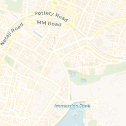
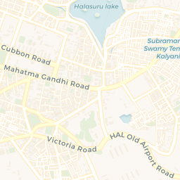
It is possible to create a list of icons, so that different Markers can have different icons. Let us try to map the MNCs in the ITPL area of Bangalore: we use the ideas in [Using Leaflet Markers @JLA-Data.net](https://www.jla-data.net/eng/leaflet-markers-in-r/)
# Make a dataframe of addresses of Companies we wan to plot in ITPL
companies_itpl <-
data.frame(
ticker = c(
"MBRDI",
"DTICI",
"IBM",
"Exxon",
"Mindtree",
"FIS Global",
"Sasken",
"LTI"
),
lat = c(
12.986178620989264,
12.984160906190121,
12.983659088566357,
12.985112265986636,
12.983794997606187,
12.980658616215155,
12.982080447350246,
12.981338168875348
),
lon = c(
77.7270652183105,
77.72808445774321,
77.73103488768001,
77.72935046040699,
77.7227844126931,
77.72685064158782,
77.72545589289041,
77.72287024338216
)
) %>% sf::st_as_sf(coords = c("lon", "lat"), crs = 4326)
# Vanilla leaflet map
leaflet(companies_itpl) %>%
addTiles() %>%
addMarkers()


Let us make a list of logos of the Companies and use them as markers!
# a named list of rescaled icons with links to images
favicons <- iconList(
"MBRDI" = makeIcon(
iconUrl = "https://www.mercedes-benz.com/etc/designs/brandhub/frontend/static-assets/header/logo.svg%22",
iconWidth = 25, iconHeight = 25
),
"DTICI" = makeIcon(
iconUrl = "https://media-exp1.licdn.com/dms/image/C4D0BAQGzOep26lC03w/company-logo_200_200/0/1638298367374?e=2147483647&v=beta&t=mPyF4gvNhNFvd-tedbqNzJofq4q9qcw6A9z9jQeLAwc%22",
iconWidth = 45, iconHeight = 45
),
"IBM" = makeIcon(
iconUrl = "https://www.ibm.com/favicon.ico%22",
iconWidth = 25, iconHeight = 25
),
"Exxon" = makeIcon(
iconUrl = "https://corporate.exxonmobil.com/-/media/Global/Icons/logos/ExxonMobilLogoColor2x.png%22",
iconWidth = 45, iconHeight = 25
),
"Mindtree" = makeIcon(
iconUrl = "https://www.mindtree.com/themes/custom/mindtree_theme/mindtree-lnt-logo-png.png%22",
iconWidth = 75, iconHeight = 25
),
"FIS Global" = makeIcon(
iconUrl = "https://1000logos.net/wp-content/uploads/2021/09/FIS-Logo-768x432.png%22",
iconWidth = 25, iconHeight = 25
),
"Sasken" = makeIcon(
iconUrl = "https://www.sasken.com/sites/all/themes/sasken_website/logo.png%22",
iconWidth = 35, iconHeight = 35,
),
"LTI" = makeIcon(
iconUrl = "https://www.lntinfotech.com/wp-content/uploads/2021/09/LTI-logo.svg%22",
iconWidth = 25, iconHeight = 25
)
)
# Create the Leaflet map
leaflet(companies_itpl) %>%
addMarkers(
icon = ~ favicons[ticker], # lookup based on ticker
label = ~ companies_itpl$ticker,
labelOptions = labelOptions(noHide = F, offset = c(15, -25))
) %>%
addProviderTiles("CartoDB.Positron")


Points using sf objects
We will use data from an sf data object. This differs from the earlier situation where we had a simple data frame with lon and lat columns. In sf, the lon and lat info is embedded in the geometry column of the sf data frame.
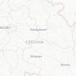
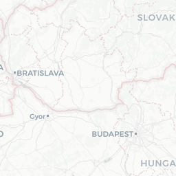
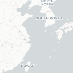
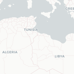
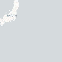
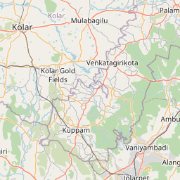
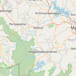
The tmap package has a data set of all World metro cities, titled metro. We will plot these on the map and also scale the markers in proportion to one of the feature attributes, pop2030. The popup will be the name of the metro city. We will also use the CartoDB.Positron base map.
Note that the metro data set has a POINT geometry, as needed!
data(metro, package = "tmap")
metroname <chr> | name_long <chr> | iso_a3 <chr> | pop1950 <dbl> | pop1960 <dbl> | pop1970 <dbl> | pop1980 <dbl> | pop1990 <dbl> | pop2000 <dbl> | ||
|---|---|---|---|---|---|---|---|---|---|---|
| 2 | Kabul | Kabul | AFG | 170784 | 285352 | 471891 | 977824 | 1549320 | 2401109 | |
| 8 | Algiers | El Djazair (Algiers) | DZA | 516450 | 871636 | 1281127 | 1621442 | 1797068 | 2140577 | |
| 13 | Luanda | Luanda | AGO | 138413 | 219427 | 459225 | 771349 | 1390240 | 2591388 | |
| 16 | Buenos Aires | Buenos Aires | ARG | 5097612 | 6597634 | 8104621 | 9422362 | 10513284 | 12406780 | |
| 17 | Cordoba | Cordoba | ARG | 429249 | 605309 | 809794 | 1009521 | 1200168 | 1347561 | |
| 25 | Rosario | Rosario | ARG | 554483 | 671349 | 816230 | 953491 | 1083819 | 1152387 | |
| 32 | Yerevan | Yerevan | ARM | 341432 | 537759 | 778158 | 1041587 | 1174524 | 1111301 | |
| 33 | Adelaide | Adelaide | AUS | 429277 | 571822 | 850168 | 971856 | 1081618 | 1141623 | |
| 34 | Brisbane | Brisbane | AUS | 441718 | 602999 | 904777 | 1134833 | 1381306 | 1666203 | |
| 37 | Melbourne | Melbourne | AUS | 1331966 | 1851220 | 2499109 | 2839019 | 3154314 | 3460541 |
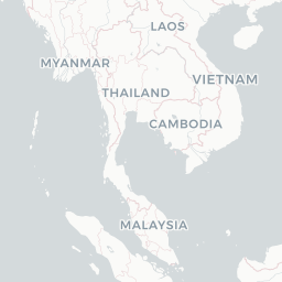
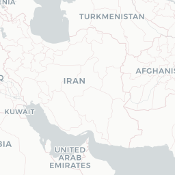
leaflet(data = metro) %>%
setView(lat = 18, lng = 77, zoom = 4) %>%
# Add CartoDB.Positron
addProviderTiles(providers$CartoDB.Positron) %>% # CartoDB Basemap
# Add Markers for each airport
addCircleMarkers(
radius = ~ sqrt(pop2030) / 350,
color = "red",
popup = paste(
"Name: ", metro$name, "<br>",
"Population 2030: ", metro$pop2030
)
)


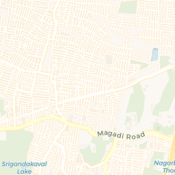
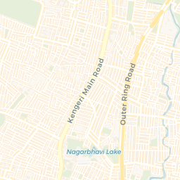
We can also try downloading an sf data frame with POINT geometry from say OSM datahttps://osm. Let us get hold of restaurants data in Malleswaram, Bangalore from OSM data:
bbox <- osmdata::getbb("Malleswaram, Bengaluru")
bbox min max
x 77.55033 77.59033
y 12.98274 13.02274locations <-
osmdata::opq(bbox = bbox) %>%
osmdata::add_osm_feature(key = "amenity", value = "restaurant") %>%
osmdata_sf() %>%
purrr::pluck("osm_points") %>%
dplyr::select(name, cuisine, geometry) %>%
dplyr::filter(cuisine == "indian")
locations %>% head()name <chr> | cuisine <chr> | geometry <sf_POINT> | ||
|---|---|---|---|---|
| 461539222 | Adiga's | indian | <sf_POINT> | |
| 598500940 | Udupi Sri Krishnarajathadri | indian | <sf_POINT> | |
| 673377213 | Sana Di Ge | indian | <sf_POINT> | |
| 673860152 | New Shanthi Sagar | indian | <sf_POINT> | |
| 1116484556 | Kabab Studio | indian | <sf_POINT> | |
| 1448082496 | Sai Shakti | indian | <sf_POINT> |
# Fontawesome icons seem to work in `leaflet` only up to FontAwesome V4.7.0.
# The Fontawesome V4.7.0 Cheatsheet is here: <https://fontawesome.com/v4/cheatsheet/>
leaflet(
data = locations,
options = leafletOptions(minZoom = 12)
) %>%
addProviderTiles(providers$CartoDB.Voyager) %>%
# Regular `leaflet` code
addAwesomeMarkers(
icon = awesomeIcons(
icon = "fa-coffee",
library = "fa",
markerColor = "blue",
iconColor = "black",
iconRotate = TRUE
),
popup = paste(
"Name: ", locations$name, "<br>",
"Food: ", locations$cuisine
)
)


Fontawesome Workaround
For more later versions of Fontawesome, here below is a workaround from https://github.com/rstudio/leaflet/issues/691. Despite this some fontawesome icons simply do not seem to show up. ;-()
library(fontawesome)
coffee <- makeAwesomeIcon(
text = fa("mug-hot"), # mug-hot was introduced in fa version 5
iconColor = "black",
markerColor = "blue",
library = "fa"
)
leaflet(data = locations) %>%
addProviderTiles(providers$CartoDB.Voyager) %>%
# Workaround code
addAwesomeMarkers(
icon = coffee,
popup = paste(
"Name: ", locations$name, "<br>",
"Food: ", locations$cuisine, "<br>"
)
)Note that leaflet automatically detects the lon/lat columns from within the POINT geometry column of the sf data frame.
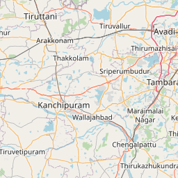
Points using Two-Column Matrices
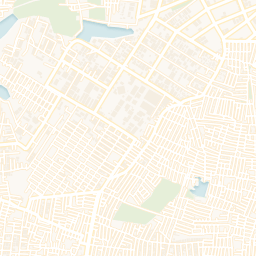
We can now quickly try providing lon and lat info in a two column matrix.This can be useful to plot a bunch of points recorded on a mobile phone app.
mysore5 <- matrix(
c(
runif(5, 76.652985 - 0.01, 76.652985 + 0.01),
runif(5, 12.311827 - 0.01, 12.311827 + 0.01)
),
nrow = 5
)
mysore5 [,1] [,2]
[1,] 76.65610 12.31230
[2,] 76.64559 12.31040
[3,] 76.64655 12.30804
[4,] 76.64881 12.30683
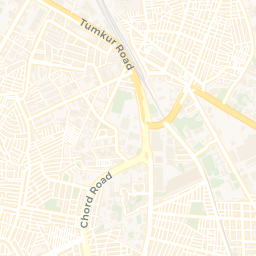
[5,] 76.66169 12.31110leaflet(data = mysore5) %>%
addProviderTiles(providers$OpenStreetMap) %>%
# Pick an icon from <https://www.w3schools.com/bootstrap/bootstrap_ref_comp_glyphs.asp>
addAwesomeMarkers(
icon = awesomeIcons(
icon = "music",
iconColor = "black",
library = "glyphicon"
),
popup = "Carnatic Music !!"
)


Leaflet | © OpenStreetMap contributors
Polygons, Lines, and Polylines Data Sources for leaflet
We have seen how to get POINT data into leaflet.
Line and polygon data can come from a variety of sources:
SpatialPolygons,SpatialPolygonsDataFrame,Polygons, andPolygon objects(from thesppackage)SpatialLines,SpatialLinesDataFrame,Lines, andLine objects(from thesppackage)MULTIPOLYGON,POLYGON,MULTILINESTRING, andLINESTRINGobjects (from thesfpackage)mapobjects (from themapspackage’smap()function); usemap(fill = TRUE)for polygons,FALSEfor polylinesTwo-column numeric
matrix; the first column is longitude and the second is latitude. Polygons are separated by rows of (NA, NA). It is not possible to represent multi-polygons nor polygons with holes using this method; useSpatialPolygonsinstead.
We will concentrate on using sf data into leaflet. We may explore maps() objects at a later date.
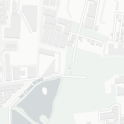
Polygons/MultiPolygons and LineString/MultiLineString using sf data frames
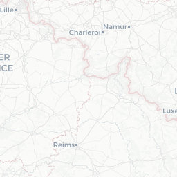
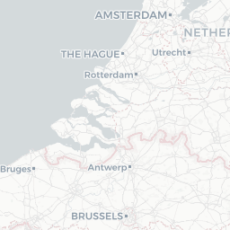
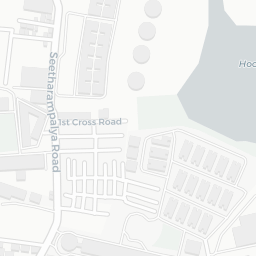
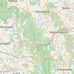
Let us download College buildings, parks, and the cycling lanes in Amsterdam, Netherlands, and plot these in leaflet.
library(osmdata)
# Option 1
# Gives too large a bbox
bbox <- osmdata::getbb("Amsterdam, Netherlands")
# bbox
# Setting bbox manually is better
amsterdam_coords <- matrix(c(4.85, 4.95, 52.325, 52.375),
byrow = TRUE,
nrow = 2, ncol = 2,
dimnames = list(c("x", "y"), c("min", "max"))
)
amsterdam_coords min max
x 4.850 4.950
y 52.325 52.375colleges <- amsterdam_coords %>%
osmdata::opq() %>%
osmdata::add_osm_feature(
key = "amenity",
value = "college"
) %>%
osmdata_sf() %>%
purrr::pluck("osm_polygons")
parks <- amsterdam_coords %>%
osmdata::opq() %>%
osmdata::add_osm_feature(key = "landuse", value = "grass") %>%
osmdata_sf() %>%
purrr::pluck("osm_polygons")
roads <- amsterdam_coords %>%
osmdata::opq() %>%
osmdata::add_osm_feature(
key = "highway",
value = "primary"
) %>%
osmdata_sf() %>%
purrr::pluck("osm_lines")
cyclelanes <- amsterdam_coords %>%
osmdata::opq() %>%
osmdata::add_osm_feature(key = "cycleway") %>%
osmdata_sf() %>%
purrr::pluck("osm_lines")We have 12 colleges in our data and 3372 parks in our data.
leaflet() %>%
addTiles() %>%
addPolygons(data = colleges, popup = ~ colleges$name) %>%
addPolygons(data = parks, color = "green", popup = parks$name) %>%
addPolylines(data = roads, color = "red") %>%
addPolylines(data = cyclelanes, color = "purple")


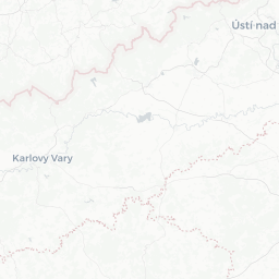
Chapter 3: Using Raster Data in leaflet
So far all the geospatial data we have plotted in leaflet has been vector data. We will now explore how to plot raster data using leaflet. Raster data are used to depict continuous variables across space, such as vegitation, salinity, forest cover etc. Satellite imagery is frequently available as raster data.
Importing Raster Data [Work in Progress!]
Raster data can be imported into R in many ways:
using the
maptilespackageusing the
OpenStreetMappackage
Bells and Whistles in leaflet: layers, groups, legends, and graticules
Adding Legends[Work in Progress!]
## Generate some random lat lon data around Bangalore
df <- data.frame(
lat = runif(20, min = 11.97, max = 13.07),
lng = runif(20, min = 77.48, max = 77.68),
col = sample(c("red", "blue", "green"), 20,
replace = TRUE
),
stringsAsFactors = FALSE
)
df %>%
leaflet() %>%
addTiles() %>%
addCircleMarkers(color = df$col) %>%
addLegend(values = df$col, labels = LETTERS[1:3], colors = c("blue", "red", "green"))


Using Web Map Services (WMS) [Work in Progress!]
To be included.