Tutorial: Multiple Linear Regression with Forward Selection

Linear Regression

Quantitative Predictor

Quantitative Response

Sum of Squares

Residuals

Author

Arvind V.

Published

May 13, 2023

Modified

May 21, 2024

Abstract

Using Multiple Regression to predict Quantitative Target Variables

Setting up R Packages

options(scipen = 1, digits = 3) #set to three decimal 
knitr::opts_chunk$set(echo = TRUE,warning = FALSE,message = FALSE) 
library(tidyverse)
library(ggformula)
library(mosaic)
library(GGally)
library(corrgram)
library(corrplot)
library(broom)

# datasets
library(ISLR)

# Let us set a plot theme for Data visualization

theme_set(theme_light(base_size = 11, base_family = "Roboto Condensed"))

theme_update(
  panel.grid.minor = element_blank(),
  plot.title = element_text(face = "bold"),
  plot.title.position = "plot"
)

In this tutorial, we will use the ~~Boston housing~~ Hitters dataset(s) from the ISLR package. Our research question is:

Research Question

How do we predict the Salary of baseball players based on other Quantitative parameters such as Hits, HmRun AtBat?

And how do we choose the “best” model, based on a trade-off between Model Complexity and Model Accuracy?

Workflow Plan

Our target variable is Salary.

We will start with an examination of correlations between Salary and other Quant predictors.

We will use a null model for our Linear Regression at first, keeping just an intercept term. Based on the examination of the r-square improvement offered by each predictor individually, we will add another quantitative predictor. We will follow this process through up to a point where the gains in model accuracy are good enough to justify the additional model complexity.

Note

This approach is the exact opposite of the earlier tutorial on multiple linear regression, where we started with a maximal model and trimmed it down based on an assessment of r.squared.

Workflow: EDA

The Hitters dataset has the following variables:

data("Hitters")
inspect(Hitters)


categorical variables:  
       name  class levels   n missing
1    League factor      2 322       0
2  Division factor      2 322       0
3 NewLeague factor      2 322       0
                                   distribution
1 A (54.3%), N (45.7%)                         
2 W (51.2%), E (48.8%)                         
3 A (54.7%), N (45.3%)                         

quantitative variables:  
      name   class  min    Q1 median     Q3   max    mean      sd   n missing
1    AtBat integer 16.0 255.2  379.5  512.0   687  380.93  153.40 322       0
2     Hits integer  1.0  64.0   96.0  137.0   238  101.02   46.45 322       0
3    HmRun integer  0.0   4.0    8.0   16.0    40   10.77    8.71 322       0
4     Runs integer  0.0  30.2   48.0   69.0   130   50.91   26.02 322       0
5      RBI integer  0.0  28.0   44.0   64.8   121   48.03   26.17 322       0
6    Walks integer  0.0  22.0   35.0   53.0   105   38.74   21.64 322       0
7    Years integer  1.0   4.0    6.0   11.0    24    7.44    4.93 322       0
8   CAtBat integer 19.0 816.8 1928.0 3924.2 14053 2648.68 2324.21 322       0
9    CHits integer  4.0 209.0  508.0 1059.2  4256  717.57  654.47 322       0
10  CHmRun integer  0.0  14.0   37.5   90.0   548   69.49   86.27 322       0
11   CRuns integer  1.0 100.2  247.0  526.2  2165  358.80  334.11 322       0
12    CRBI integer  0.0  88.8  220.5  426.2  1659  330.12  333.22 322       0
13  CWalks integer  0.0  67.2  170.5  339.2  1566  260.24  267.06 322       0
14 PutOuts integer  0.0 109.2  212.0  325.0  1378  288.94  280.70 322       0
15 Assists integer  0.0   7.0   39.5  166.0   492  106.91  136.85 322       0
16  Errors integer  0.0   3.0    6.0   11.0    32    8.04    6.37 322       0
17  Salary numeric 67.5 190.0  425.0  750.0  2460  535.93  451.12 263      59

Scatter Plots and Correlations

We should examine scatter plots and Correlations of Salary against these variables. Let us select a few sets of Quantitative and Qualitative features, along with the target variable Salary and do a pairs-plots with them:

Hitters %>% 
  select(Salary, AtBat, Hits, HmRun) %>% 
  GGally::ggpairs(title = "Plot 1", lower = list(continuous = wrap("smooth", alpha = 0.2)))
Hitters %>% 
  select(Salary, Runs, RBI, Walks,Years) %>% 
  GGally::ggpairs(title = "Plot 2", lower = list(continuous = wrap("smooth", alpha = 0.2)))
Hitters %>% 
  select(Salary, CRBI, CAtBat, CHits, CHmRun, CRuns, CWalks) %>% 
  GGally::ggpairs(title = "Plot 3", lower = list(continuous = wrap("smooth", alpha = 0.2)))
Hitters %>% 
  select(Salary, PutOuts,Assists,Errors) %>% 
  GGally::ggpairs(title = "Plot 4", lower = list(continuous = wrap("smooth", alpha = 0.2)))
Hitters %>% 
  select(Salary, League,Division,NewLeague) %>% 
  GGally::ggpairs(title = "Plot 5", lower = list(continuous = wrap("smooth", alpha = 0.2)))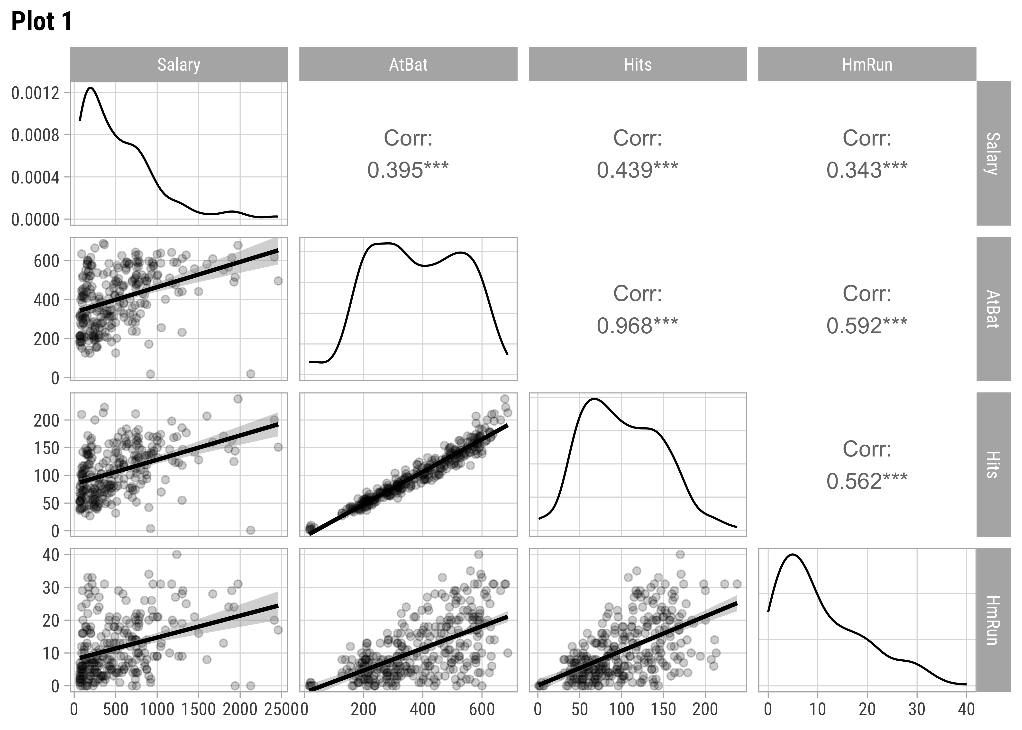

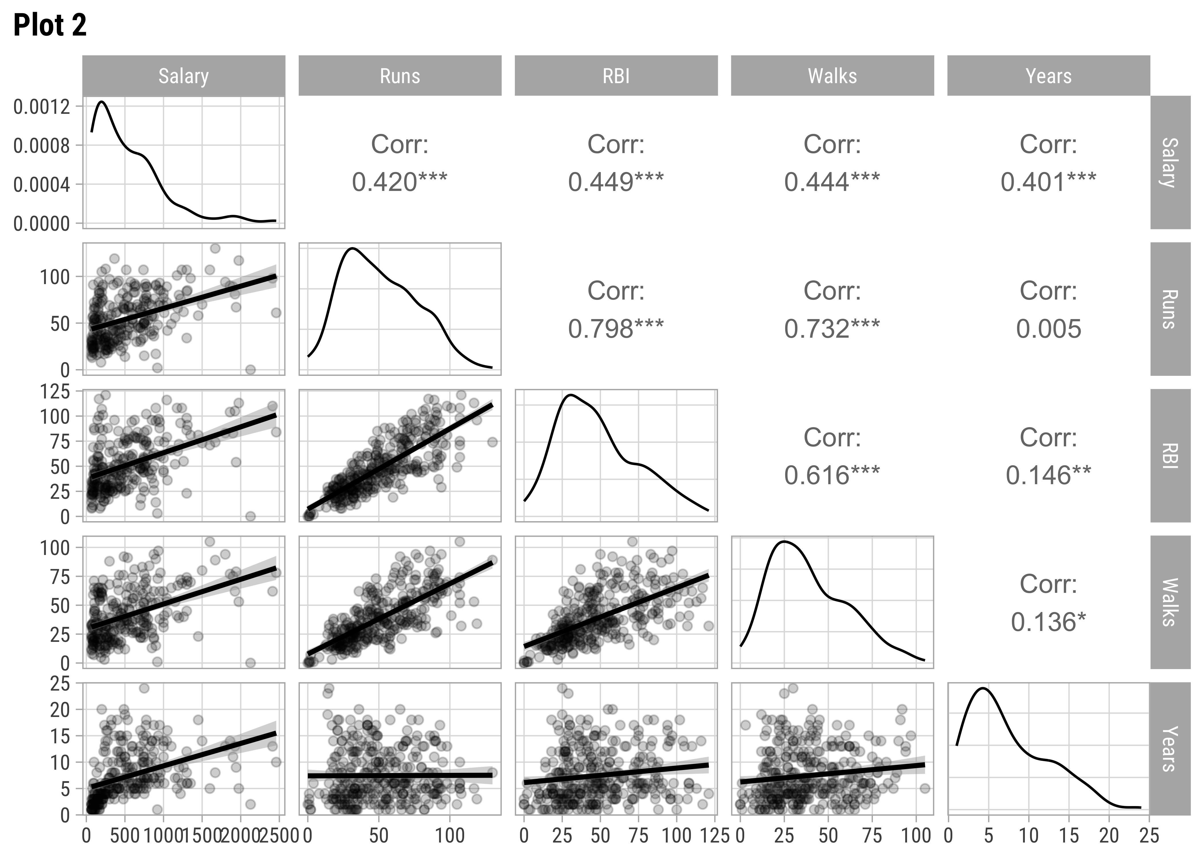
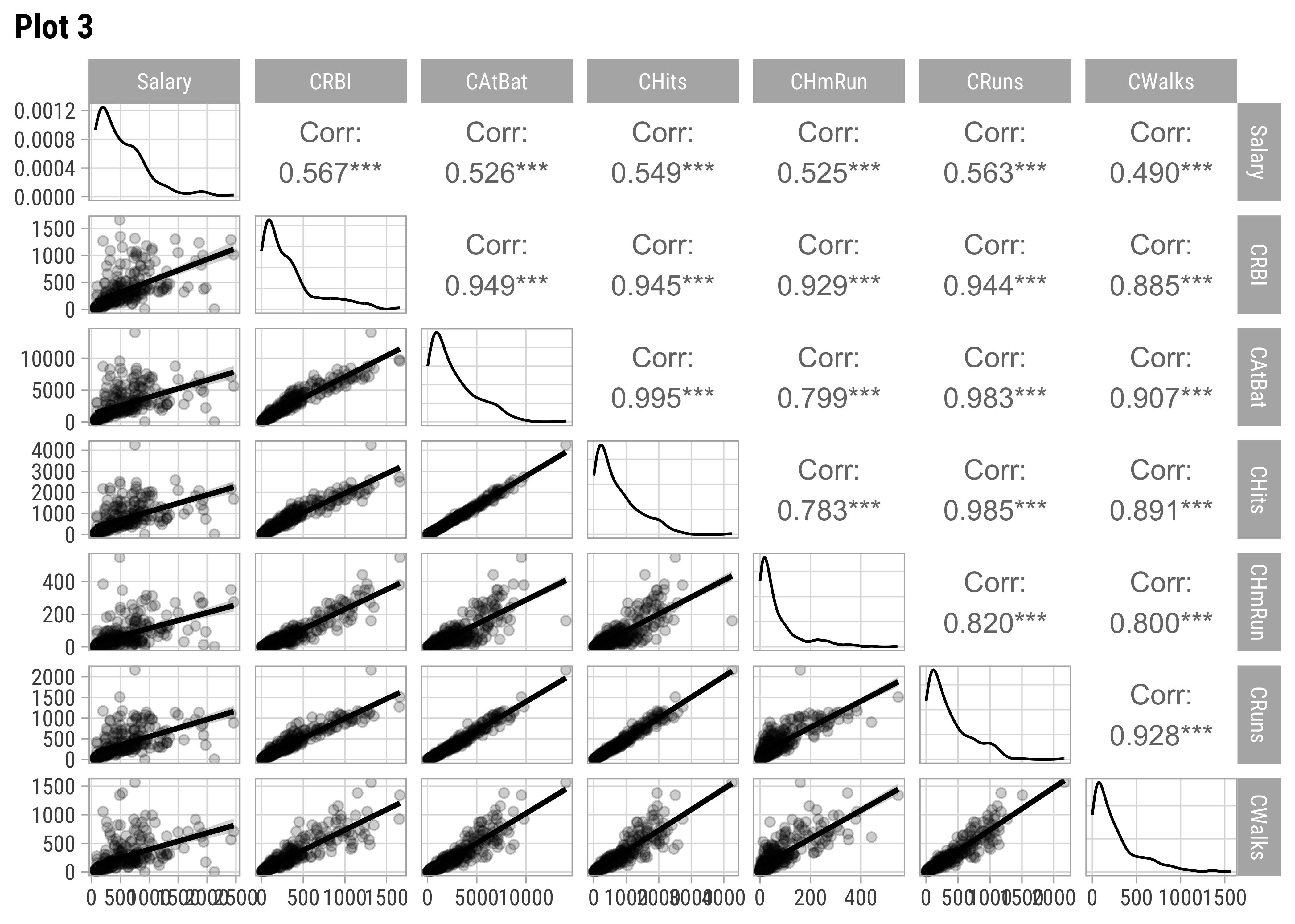
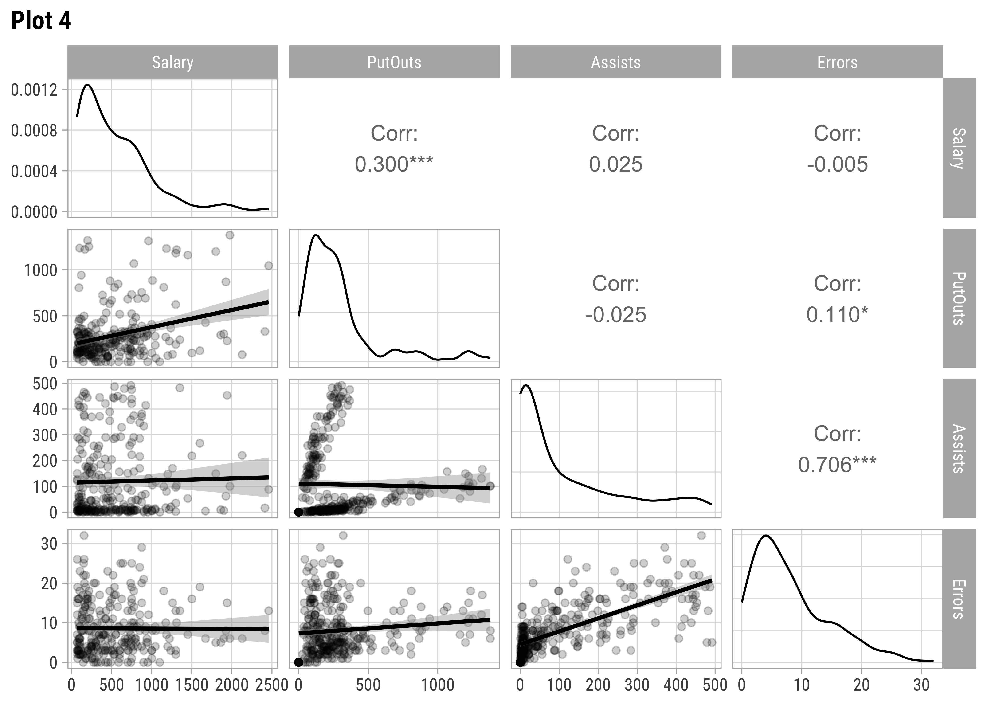
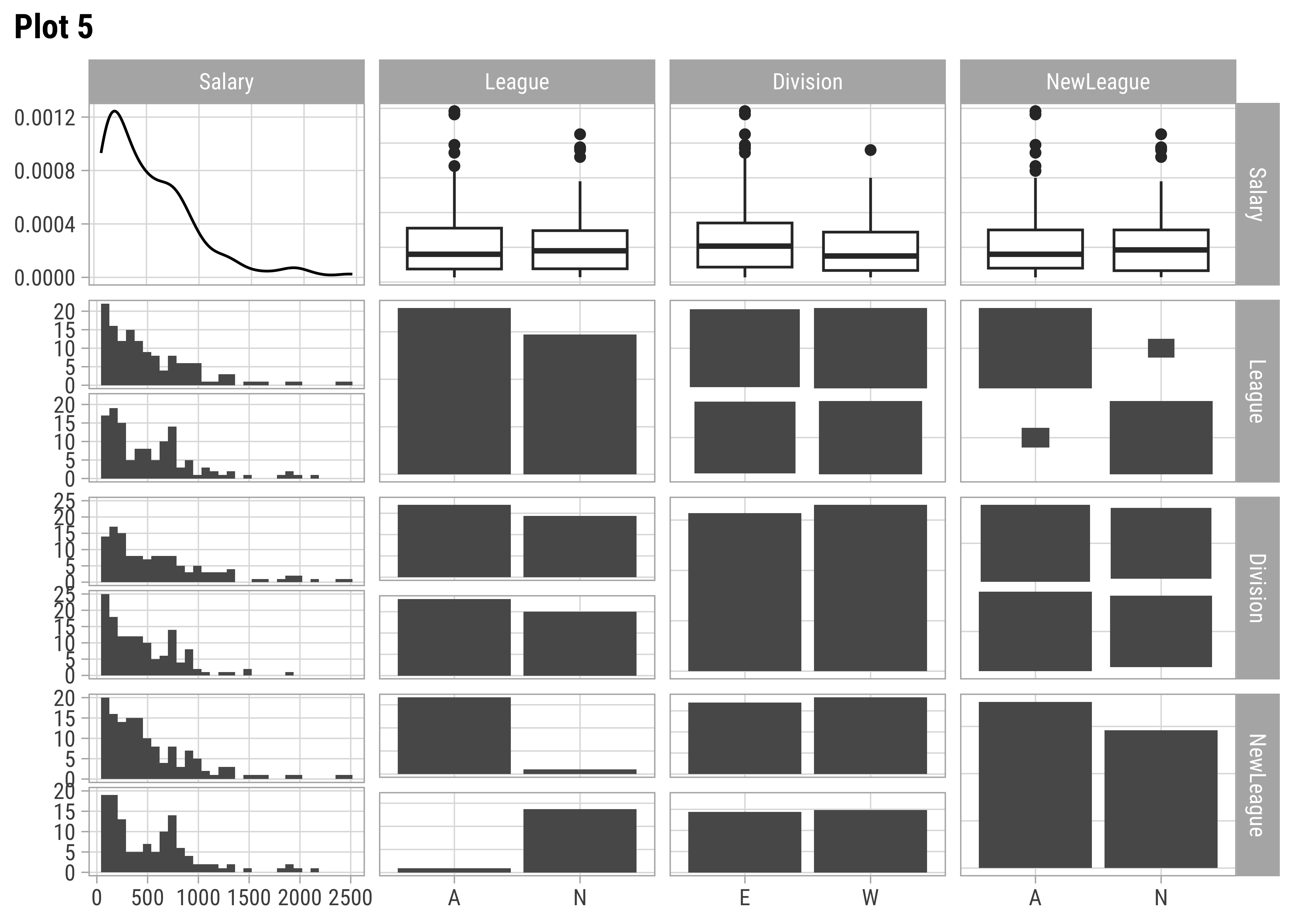
AtBat and Hits seem relevant predictors for Salary. So are Runs, RBI,Walks, and Years. From Plot 2, both RBI and Walks are also inter-correlated with Runs. All the C* variables are well correlated with Salary and also among one another. (Plot3). Plot 4 has no significant correlations at all. Plot 5 shows Salary nearly equally distributed across League, Division, and NewLeague.

Correlation Error-Bars

We can also plot all correlations in one graph using cor.test and purrr:

all_corrs <- 
  Hitters %>% 
  select(where(is.numeric)) %>% 
  
  # leave off Salary and year to get all the remaining ones
  select(- Salary) %>% 
  
  
  # perform a cor.test for all variables against Salary
  purrr::map(.x = .,
             .f = \(x) cor.test(x, Hitters$Salary)) %>%
  
  # tidy up the cor.test outputs into a tidy data frame
  map_dfr(broom::tidy, .id = "predictor") %>% 
  arrange(desc(estimate))

all_corrs
all_corrs %>%
  gf_hline(yintercept = 0,
           linewidth = 2,
           color = "grey") %>%
  gf_errorbar(
    conf.high + conf.low ~ reorder(predictor, estimate),
    color = ~ estimate,
    linewidth =  ~ -log10(p.value),
    width = 0.5,
    caption = "Significance = -log10(p.value)"
  ) %>%
  gf_point(estimate ~ reorder(predictor, estimate)) %>%
  gf_labs(x = NULL, y = "Correlation with Salary") %>%
  #gf_theme(theme = my_theme()) %>%
  gf_refine(
    scale_colour_distiller("Correlation", type = "div",
                           palette = "RdBu"),
    scale_linewidth_continuous("Significance", range = c(0.25, 3))
  ) %>%
  gf_refine(guides(linewidth = guide_legend(reverse = TRUE)),
            theme(axis.text.x = element_text(hjust = 1))) %>%
  gf_refine(guides(linewidth = guide_legend(reverse = TRUE)),
            coord_flip())

ABCDEFGHIJ0123456789

predictor <chr>	estimate <dbl>	statistic <dbl>	p.value <dbl>	parameter <int>
CRBI	0.5670	11.1195	9.07e-24	261
CRuns	0.5627	10.9962	2.31e-23	261
CHits	0.5489	10.6090	4.26e-22	261
CAtBat	0.5261	9.9953	3.98e-20	261
CHmRun	0.5249	9.9637	5.01e-20	261
CWalks	0.4898	9.0768	2.82e-17	261
RBI	0.4495	8.1285	1.76e-14	261
Walks	0.4439	8.0024	4.01e-14	261
Hits	0.4387	7.8863	8.53e-14	261
Runs	0.4199	7.4737	1.18e-12	261

There are a good many predictors which have statistically significant correlations with Salary, such as CRuns , CHmRun. The darker the colour, the higher is the correlation score; the fatter the bar, the higher is the significance of the correlation.

We now start with setting up simple Linear Regressions with no predictors, only an intercept. We then fit separate Linear Models using each predictor individually. Then based on the the improvement in r.squared offered by each predictor, we progressively add it to the model, until we are “satisfied” with the quality of the model ( using rsquared and other means).

Let us now do this.

Workflow: Minimal Multiple Regression Model

Note the formula structure here: we want just and intercept.

lm_min <- lm(data = Hitters, Salary ~ 1)
summary(lm_min)


Call:
lm(formula = Salary ~ 1, data = Hitters)

Residuals:
   Min     1Q Median     3Q    Max 
  -468   -346   -111    214   1924 

Coefficients:
            Estimate Std. Error t value Pr(>|t|)    
(Intercept)    535.9       27.8    19.3   <2e-16 ***
---
Signif. codes:  0 '***' 0.001 '**' 0.01 '*' 0.05 '.' 0.1 ' ' 1

Residual standard error: 451 on 262 degrees of freedom
  (59 observations deleted due to missingness)

lm_min %>% broom::tidy()
lm_min %>% broom::glance()

ABCDEFGHIJ0123456789

term <chr>	estimate <dbl>	std.error <dbl>	statistic <dbl>	p.value <dbl>
(Intercept)	536	27.8	19.3	4.02e-52

ABCDEFGHIJ0123456789

r.squared <dbl>	adj.r.squared <dbl>	sigma <dbl>	statistic <dbl>	p.value <dbl>	df <dbl>
0	0	451	NA	NA	NA

OK, so the intercept is highly significant, the t-statistic is also high, but the intercept contributes nothing to the r.squared!! It is of no use at all!

Workflow: Predictor Addition (Round#1)

We will now set up individual models for each predictor and look at the p.value and r.squared offered by each separate model:

names <- names(Hitters %>%
  select(where(is.numeric), 
         -c(Salary)))

n_vars <- length(names)

Hitters_model_set <- tibble(all_vars = list(names),
                            keep_vars = seq(1, n_vars),
                            data = list(Hitters))

# Unleash purrr in a series of mutates
Hitters_model_set <- Hitters_model_set %>%
  
# Select Single Predictor for each Simple Model
  mutate(mod_vars =
           pmap(
             .l = list(all_vars, keep_vars, data),
             .f = \(all_vars, keep_vars, data) all_vars[keep_vars]
           )) %>%
  
# build formulae with these for linear regression
  mutate(formula = map(.x = mod_vars,
                       .f = \(mod_vars) as.formula(paste(
                         "Salary ~", paste(mod_vars, collapse = "+")
                       )))) %>%
  
# use the formulae to build multiple linear models
  mutate(models =
           pmap(
             .l = list(data, formula),
             .f = \(data, formula) lm(formula, data = data)
           ))


# Tidy up the models using broom to expose their metrics
Hitters_model_set <- 
  Hitters_model_set %>% 
  mutate(tidy_models =
           map(
             .x = models,
             .f = \(x) broom::glance(x,
                                     conf.int = TRUE,
                                     conf.lvel = 0.95)
           ),
         predictor_name = names[keep_vars]) %>% 

  # Remove unwanted columns, keep model and predictor count
  select(keep_vars,predictor_name, tidy_models) %>%
  unnest(tidy_models) %>% 
  arrange(desc(r.squared))

# Check everything after the operation
Hitters_model_set
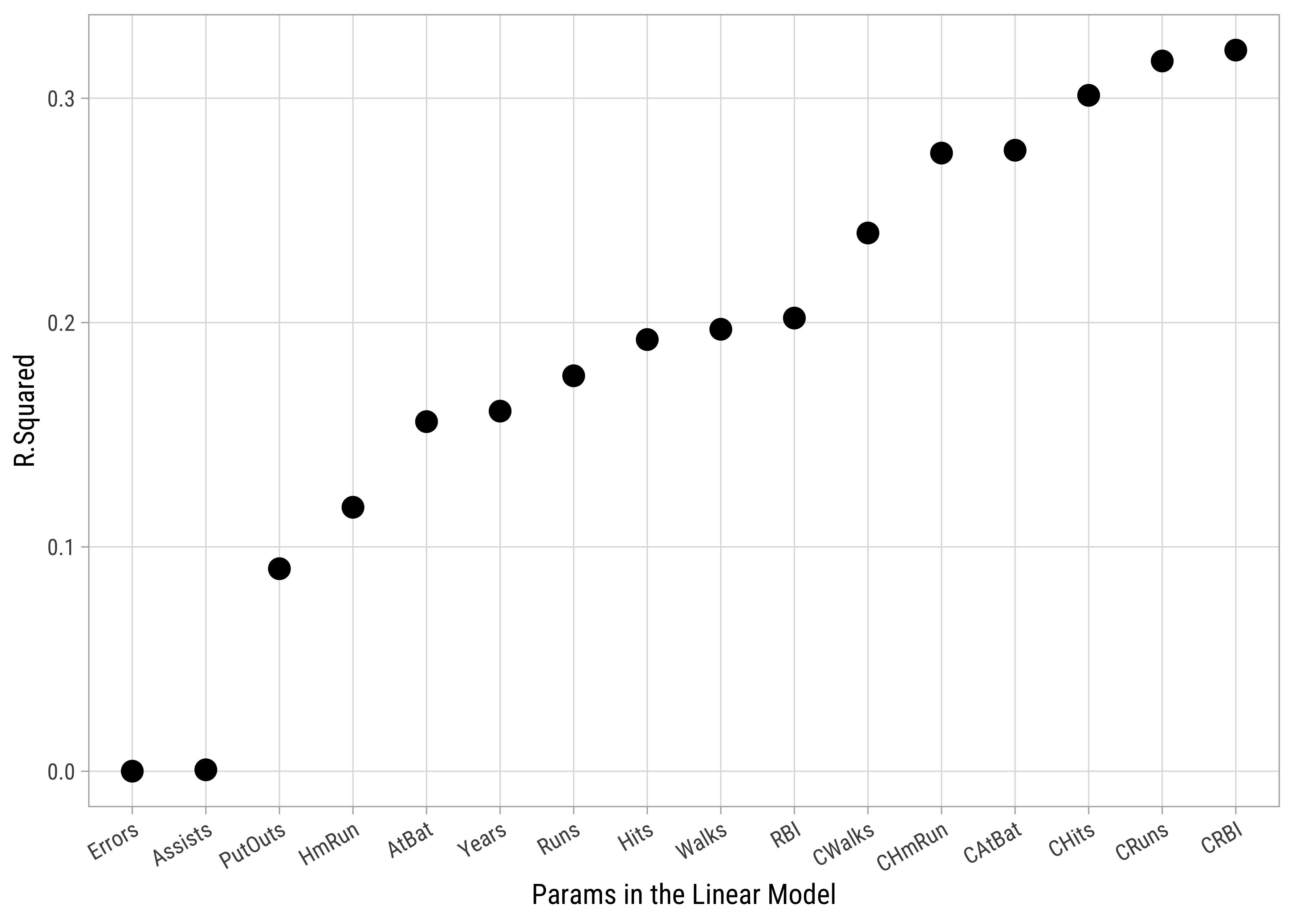
# Plot r.squared vs predictor count
Hitters_model_set %>% 
  gf_point(r.squared ~ reorder(predictor_name, r.squared), 
           size = 3.5, 
           color = "black",
           ylab = "R.Squared",
           xlab = "Params in the Linear Model", data = .) %>%
  #gf_theme(my_theme()) %>% 
  gf_refine(theme(axis.text.x = element_text(angle = 30,
                                             hjust = 1)))

ABCDEFGHIJ0123456789

keep_vars <int>	predictor_name <chr>	r.squared <dbl>	adj.r.squared <dbl>
12	CRBI	0.3214501	0.31885
11	CRuns	0.3166062	0.31399
9	CHits	0.3013017	0.29862
8	CAtBat	0.2768184	0.27405
10	CHmRun	0.2755521	0.27278
13	CWalks	0.2399256	0.23701
5	RBI	0.2020117	0.19895
6	Walks	0.1970181	0.19394
2	Hits	0.1924355	0.18934
4	Runs	0.1762812	0.17313

# Which is the winning Predictor?
winner <- Hitters_model_set %>% 
  arrange(desc(r.squared)) %>% 
  select(predictor_name) %>% 
  head(1) %>% as.character()
winner

[1] "CRBI"

# Here is the Round 1 Model
# Minimal model updated to included winning predictor
lm_round1 <- update(lm_min, ~. + CRBI)
lm_round1 %>% broom::tidy()
lm_round1 %>% broom::glance()

ABCDEFGHIJ0123456789

term <chr>	estimate <dbl>	std.error <dbl>	statistic <dbl>	p.value <dbl>
(Intercept)	274.580	32.8554	8.36	3.85e-15
CRBI	0.791	0.0711	11.12	9.07e-24

ABCDEFGHIJ0123456789

r.squared <dbl>	adj.r.squared <dbl>	sigma <dbl>	statistic <dbl>	p.value <dbl>	df <dbl>
0.321	0.319	372	124	9.07e-24	1

So we can add CRBI as a predictor to our model as a predictor gives us an improved r.squared of $0.321$ , which is the square of the correlation between Salary and CRBI, $.567$ .

And the model itself is: $\begin{matrix} (1) & S a l a r y \sim 274.580 + 0.791 \times C R B I \end{matrix}$

Let’s press on to Round 2.

Workflow: Predictor Addition (Round #2)

We will set up a round-2 model using CRBI as the predictor, and then proceed to add each of the other predictors as an update to the model.

# Preliminaries
names <- names(Hitters %>%
  select(where(is.numeric), -c(Salary, winner)))
# names

n_vars <- length(names)
# n_vars
# names <- names %>% str_remove(winner)
# names
# n_vars <- n_vars-1


# Round 2 Iteration
Hitters_model_set <- tibble(all_vars = list(names),
                            keep_vars = seq(1, n_vars),
                            data = list(Hitters))
# Hitters_model_set 

# Unleash purrr in a series of mutates
Hitters_model_set <- Hitters_model_set %>%
  
# list of predictor variables for each model
  mutate(mod_vars =
           pmap(
             .l = list(all_vars, keep_vars, data),
             .f = \(all_vars, keep_vars, data) all_vars[keep_vars]
           )) %>%
  
# build formulae with these for linear regression
  mutate(formula = map(.x = mod_vars,
                       .f = \(mod_vars) as.formula(paste(
                         "Salary ~ CRBI +", paste(mod_vars, collapse = "+")
                       )))) %>%
  
# use the formulae to build multiple linear models
  mutate(models =
           pmap(
             .l = list(data, formula),
             .f = \(data, formula) lm(formula, data = data)
           ))
# Check everything after the operation
# Hitters_model_set

# Tidy up the models using broom to expose their metrics
Hitters_model_set <- 
  Hitters_model_set %>% 
  mutate(tidy_models =
           map(
             .x = models,
             .f = \(x) broom::glance(x,
                                     conf.int = TRUE,
                                     conf.lvel = 0.95)
           ),
         predictor_name = names[keep_vars]) %>% 

  # Remove unwanted columns, keep model and predictor count
  select(keep_vars,predictor_name, tidy_models) %>%
  unnest(tidy_models) %>% 
  arrange(desc(r.squared))

Hitters_model_set
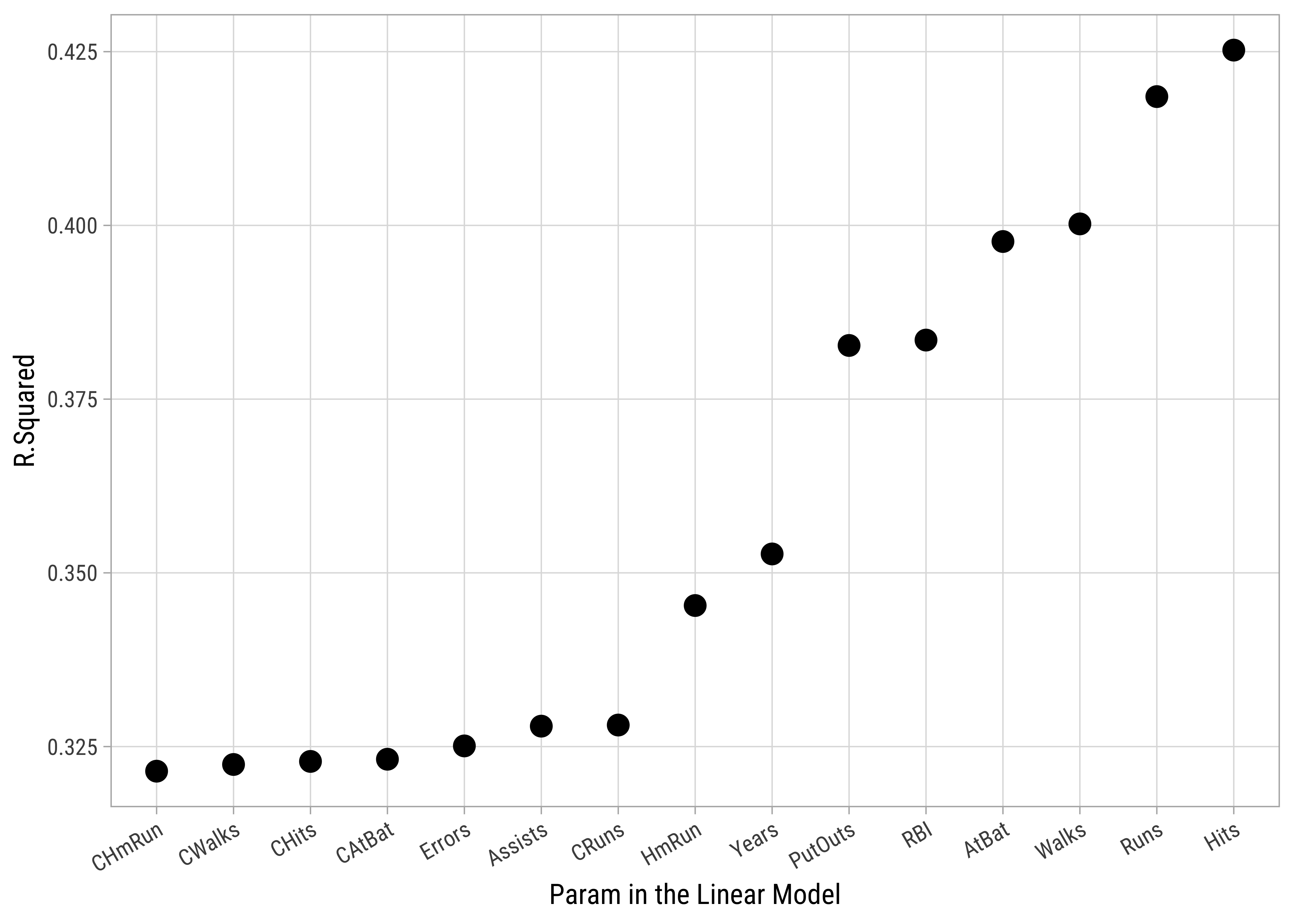
# Plot r.squared vs predictor count
Hitters_model_set %>% 
  gf_point(r.squared ~ reorder(predictor_name, r.squared), 
                               size = 3.5,
                               ylab = "R.Squared",
                               xlab = "Param in the Linear Model") %>%
  #gf_theme(my_theme()) %>% 
  gf_refine(theme(axis.text.x = element_text(angle = 30, 
                                             hjust = 1)))

ABCDEFGHIJ0123456789

keep_vars <int>	predictor_name <chr>	r.squared <dbl>	adj.r.squared <dbl>
2	Hits	0.425	0.421
4	Runs	0.419	0.414
6	Walks	0.400	0.396
1	AtBat	0.398	0.393
5	RBI	0.383	0.379
13	PutOuts	0.383	0.378
7	Years	0.353	0.348
3	HmRun	0.345	0.340
11	CRuns	0.328	0.323
14	Assists	0.328	0.323

# Which is the winning Predictor?
# 
winner <- Hitters_model_set %>% 
  arrange(desc(r.squared)) %>% 
  select(predictor_name) %>% 
  head(1) %>% as.character()
winner
# Here is the Round 1 Model
lm_round2 <- update(lm_round1, ~. + Hits)
lm_round2 %>% broom::tidy()
lm_round2 %>% broom::glance()

[1] "Hits"

ABCDEFGHIJ0123456789

term <chr>	estimate <dbl>	std.error <dbl>
(Intercept)	-47.96	55.9825
CRBI	0.69	0.0672
Hits	3.30	0.4818

ABCDEFGHIJ0123456789

r.squared <dbl>	adj.r.squared <dbl>	sigma <dbl>
0.425	0.421	343

And now the model itself is: $\begin{matrix} (2) & S a l a r y \sim - 47.96 + 0.691 \times C R B I + 3.30 \times H i t s \end{matrix}$

Note the change in both intercept and the slope for CRBI when the new predictor Hits is added!!

Workflow: Visualization

Let us quickly see how this model might look. We know that with simple regression, we obtain a straight line as our model. Here, with two (or more) predictors, we should obtain a ….(hyper)plane! Play with the interactive plot below!

ABCDEFGHIJ0123456789

.rownames <chr>	Salary <dbl>	CRBI <int>	Hits <int>	.fitted <dbl>	.resid <dbl>	.hat <dbl>	.sigma <dbl>	.cooksd <dbl>	.std.resid <dbl>
-Alan Ashby	475.0	414	81	505.0	-30.03	0.00576	344	1.49e-05	-0.08772
-Alvin Davis	480.0	266	130	564.7	-84.67	0.00510	344	1.04e-04	-0.24724
-Andre Dawson	500.0	838	141	995.6	-495.60	0.01382	343	9.87e-03	-1.45361
-Andres Galarraga	91.5	46	87	271.0	-179.45	0.00704	344	6.51e-04	-0.52454
-Alfredo Griffin	750.0	336	169	741.7	8.31	0.01113	344	2.22e-06	0.02433
-Al Newman	70.0	9	37	80.4	-10.38	0.01490	344	4.68e-06	-0.03047
-Argenis Salazar	100.0	37	73	218.5	-118.53	0.00826	344	3.34e-04	-0.34668
-Andres Thomas	75.0	34	81	242.9	-167.87	0.00763	344	6.17e-04	-0.49083
-Andre Thornton	1100.0	890	92	869.7	230.27	0.01737	344	2.70e-03	0.67660
-Alan Trammell	517.1	504	159	824.6	-307.44	0.00904	343	2.46e-03	-0.89957

Discussion

It is interesting that the second variable to be added was Hits which has a lower correlation of $r = 0.439$ with Salary compared to some other Quant predictors such as Chits( $r = 0.525$ ). This is because CRBI is hugely correlated with all of these predictors, so CRBI effectively acts as a proxy for all of these. See Plot 3.

We see that adding Hits to the model gives us an improved r.squared of $0.425$ .

Conclusion

We can proceed in this way to subsequent rounds and decide to stop when the model complexity (no. of predictors ) and the resulting gain in r.squared does not seem worth it.

Automatic Iteration Method

We ought to convert the above code into an R function and run it that way for a specific number of rounds to see how things pan out. ~~That is in the next version of this Tutorial!~~ It appears that there is, what else, an R Package, called reghelper that allows us to do this! 😇 The reghelper::build_model() function can be used to:

Start with only an intercept
Sequentially add each of the other predictor variables into the model “blocks”
Blocks will be added in the order they are passed to the function, and variables from previous blocks will be included with each subsequent block, so they do not need to be repeated.

Type help(rehelper) in your Console.

library(reghelper)

big_model <- build_model(
  dv = Salary, 
  # Start with only an intercept lm(Salary ~ 1, data = .)
  
  # Sequentially add each of the other predictor variables
  # Pass through variable names (or interaction terms) to add for each block. 
  # To add one term to a block, just pass it through directly; 
  # to add multiple terms at a time to a block, pass it through in a vector or list. 
  # Interaction Terms can be specified using the vector/list
  # Blocks will be added in the order they are passed to the function
  # Variables from previous blocks will be included with each subsequent block,  so they do not need to be repeated.
  
  1, AtBat, Hits, HmRun, Runs, RBI, Walks, Years, CAtBat, CHits, 
  CHmRun, CRuns, CRBI, CWalks, PutOuts, Assists, Errors,
  
  data = Hitters, 
  model = 'lm')

This multiple model is a list object with 4 items. Type summary(big_model) in your Console.

We can clean it up a wee bit:

library(gt)
# big_model has 4 parts: formulas, residuals, coefficients, overall

overall_clean <- summary(big_model)$overall %>% as_tibble() %>% janitor::clean_names()

formulas_clean <- summary(big_model)$formulas %>% 
  as.character() %>% as_tibble() %>% 
  rename("model_formula" = value)

all_models <- cbind(formulas_clean, overall_clean) %>% 
  dplyr::select(1,2,8)
all_models %>% 
  gt::gt() %>% 
    tab_style(style = cell_fill(color = "grey"),
            locations = cells_body(rows = seq(1, 18, 2)))

model_formula	r_squared	delta_r_sq
Salary ~ 1	NA	NA
Salary ~ 1 + AtBat	0.156	NA
Salary ~ 1 + AtBat + Hits	0.204	0.047748
Salary ~ 1 + AtBat + Hits + HmRun	0.227	0.023530
Salary ~ 1 + AtBat + Hits + HmRun + Runs	0.227	0.000137
Salary ~ 1 + AtBat + Hits + HmRun + Runs + RBI	0.244	0.016807
Salary ~ 1 + AtBat + Hits + HmRun + Runs + RBI + Walks	0.307	0.062553
Salary ~ 1 + AtBat + Hits + HmRun + Runs + RBI + Walks + Years	0.409	0.101919
Salary ~ 1 + AtBat + Hits + HmRun + Runs + RBI + Walks + Years + CAtBat	0.455	0.046369
Salary ~ 1 + AtBat + Hits + HmRun + Runs + RBI + Walks + Years + CAtBat + CHits	0.471	0.016234
Salary ~ 1 + AtBat + Hits + HmRun + Runs + RBI + Walks + Years + CAtBat + CHits + CHmRun	0.488	0.016771
Salary ~ 1 + AtBat + Hits + HmRun + Runs + RBI + Walks + Years + CAtBat + CHits + CHmRun + CRuns	0.488	0.000333
Salary ~ 1 + AtBat + Hits + HmRun + Runs + RBI + Walks + Years + CAtBat + CHits + CHmRun + CRuns + CRBI	0.489	0.001157
Salary ~ 1 + AtBat + Hits + HmRun + Runs + RBI + Walks + Years + CAtBat + CHits + CHmRun + CRuns + CRBI + CWalks	0.498	0.008575
Salary ~ 1 + AtBat + Hits + HmRun + Runs + RBI + Walks + Years + CAtBat + CHits + CHmRun + CRuns + CRBI + CWalks + PutOuts	0.522	0.023739
Salary ~ 1 + AtBat + Hits + HmRun + Runs + RBI + Walks + Years + CAtBat + CHits + CHmRun + CRuns + CRBI + CWalks + PutOuts + Assists	0.527	0.005401
Salary ~ 1 + AtBat + Hits + HmRun + Runs + RBI + Walks + Years + CAtBat + CHits + CHmRun + CRuns + CRBI + CWalks + PutOuts + Assists + Errors	0.528	0.000814

So we have a list of all models with main effects only. We could play with the build_model function to develop interaction models too! Slightly weird that the NULL model of Salary~1 does not show an r.squared value with build_model…??

References

https://ethanwicker.com/2021-01-11-multiple-linear-regression-002/

R Package Citations

Package	Version	Citation
corrgram	1.14	Wright (2021)
corrplot	0.92	Wei and Simko (2021)
GGally	2.2.1	Schloerke et al. (2024)
gt	0.10.1	Iannone et al. (2024)
infer	1.0.7	Couch et al. (2021)
ISLR	1.4	James et al. (2021)
janitor	2.2.0	Firke (2023)
reghelper	1.1.2	Hughes and Beiner (2023)

Couch, Simon P., Andrew P. Bray, Chester Ismay, Evgeni Chasnovski, Benjamin S. Baumer, and Mine Çetinkaya-Rundel. 2021. “infer: An R Package for Tidyverse-Friendly Statistical Inference.” Journal of Open Source Software 6 (65): 3661. https://doi.org/10.21105/joss.03661.

Firke, Sam. 2023. janitor: Simple Tools for Examining and Cleaning Dirty Data. https://CRAN.R-project.org/package=janitor.

Hughes, Jeffrey, and David Beiner. 2023. reghelper: Helper Functions for Regression Analysis. https://CRAN.R-project.org/package=reghelper.

Iannone, Richard, Joe Cheng, Barret Schloerke, Ellis Hughes, Alexandra Lauer, and JooYoung Seo. 2024. gt: Easily Create Presentation-Ready Display Tables. https://CRAN.R-project.org/package=gt.

James, Gareth, Daniela Witten, Trevor Hastie, and Rob Tibshirani. 2021. ISLR: Data for an Introduction to Statistical Learning with Applications in r. https://CRAN.R-project.org/package=ISLR.

Schloerke, Barret, Di Cook, Joseph Larmarange, Francois Briatte, Moritz Marbach, Edwin Thoen, Amos Elberg, and Jason Crowley. 2024. GGally: Extension to “ggplot2”. https://CRAN.R-project.org/package=GGally.

Wei, Taiyun, and Viliam Simko. 2021. R Package “corrplot”: Visualization of a Correlation Matrix. https://github.com/taiyun/corrplot.

Wright, Kevin. 2021. corrgram: Plot a Correlogram. https://CRAN.R-project.org/package=corrgram.

Citation

BibTeX citation:

@online{v.2023,
  author = {V., Arvind},
  title = {Tutorial: {Multiple} {Linear} {Regression} with {Forward}
    {Selection}},
  date = {2023-05-13},
  url = {https://av-quarto.netlify.app/content/courses/Analytics/Modelling/Modules/LinReg/files/forward-selection-1.html},
  langid = {en},
  abstract = {Using Multiple Regression to predict Quantitative Target
    Variables}
}

For attribution, please cite this work as:

V., Arvind. 2023. “Tutorial: Multiple Linear Regression with Forward Selection.” May 13, 2023. https://av-quarto.netlify.app/content/courses/Analytics/Modelling/Modules/LinReg/files/forward-selection-1.html.