Lab 05: Colors with Penguins

Palettes from Famous Paintings, GoT, Harry Potter, and Wes Anderson

Author

Arvind Venkatadri

Published

July 10, 2021

Modified

May 21, 2024

Setting up R Packages

knitr::opts_chunk$set(error = TRUE, comment = NA, warning = FALSE, errors = FALSE, message = FALSE, tidy = FALSE, cache = FALSE, fig.path= "03-figs/")

library(tidyverse) # Manage data
library(scales) # Create special ( % or $ ) scales
#
library(palmerpenguins) # source of our data
#
library(RColorBrewer) # Colour Palettes
library(wesanderson) # Colour Palettes
#library(gameofthrones) # You all know this!
#
library(paletteer) # Colour Palettes
library(colorspace) # Colour Palettes
#
library(patchwork) # arranges plots on Row-Col 
library(ggthemes)

Introduction

This Quarto document is part of my Workshop in R. The material is based on A Layered Grammar of Graphics by Hadley Wickham. The course is meant for First Year students pursuing a Degree in Art and Design. The intent is to build Skill in coding in R, and also appreciate R as a way to metaphorically visualize information of various kinds, using predominantly geometric figures and structures.

All Quarto files combine code, text, web-images, and figures developed using code. Everything is text; code chunks are enclosed in fences (```)

Goals

(Re)Understand different kinds of data variables
Appreciate how they can be identified based on the Interrogative Pronouns they answer to
Understand how each kind of variable lends itself to a specific choice of colour scale in the data visualization.

Pedagogical Note

The method followed will be based on PRIMM:

PREDICT Inspect the code and guess at what the code might do, write predictions
RUN the code provided and check what happens
INFER what the parameters of the code do and write comments to explain. What bells and whistles can you see?
MODIFY the parameters code provided to understand the options available. Write comments to show what you have aimed for and achieved.
MAKE : take an idea/concept of your own, and graph it.

In the following, there is some boiler plate code demonstrating the use of colour palettes in R. There are places where YOUR TURN is mention; copy and play with the boiler plate code to see what happens !

Data

We will use the penguins dataset built into the palmerpenguins package. Your should try other datasets too!

Here is a glimpse of the data:

glimpse(penguins)

Rows: 344
Columns: 8
$ species           <fct> Adelie, Adelie, Adelie, Adelie, Adelie, Adelie, Adel…
$ island            <fct> Torgersen, Torgersen, Torgersen, Torgersen, Torgerse…
$ bill_length_mm    <dbl> 39.1, 39.5, 40.3, NA, 36.7, 39.3, 38.9, 39.2, 34.1, …
$ bill_depth_mm     <dbl> 18.7, 17.4, 18.0, NA, 19.3, 20.6, 17.8, 19.6, 18.1, …
$ flipper_length_mm <int> 181, 186, 195, NA, 193, 190, 181, 195, 193, 190, 186…
$ body_mass_g       <int> 3750, 3800, 3250, NA, 3450, 3650, 3625, 4675, 3475, …
$ sex               <fct> male, female, female, NA, female, male, female, male…
$ year              <int> 2007, 2007, 2007, 2007, 2007, 2007, 2007, 2007, 2007…

Note that the unit of observation here is one-row-per-penguin.

Variables you need for this lab:

Colour vs fill aesthetic

Fill and colour scales in ggplot2 can use the same palettes. Some shapes such as lines only accept the colour aesthetic, while others, such as polygons, accept both colour and fill aesthetics. In the latter case, the colour refers to the border of the shape, and the fill to the interior.

## A look at all 25 symbols
df <- data.frame(x = 1:5,
                 y = rep(rev(seq(0, 24, by = 5)), each = 5),
                 z = 1:25)
s <- ggplot(df, aes(x = x, y = y)) +
  geom_text(aes(label = z, y = y - 1)) +
  theme_void()
s + geom_point(aes(shape = z), size = 4) + scale_shape_identity()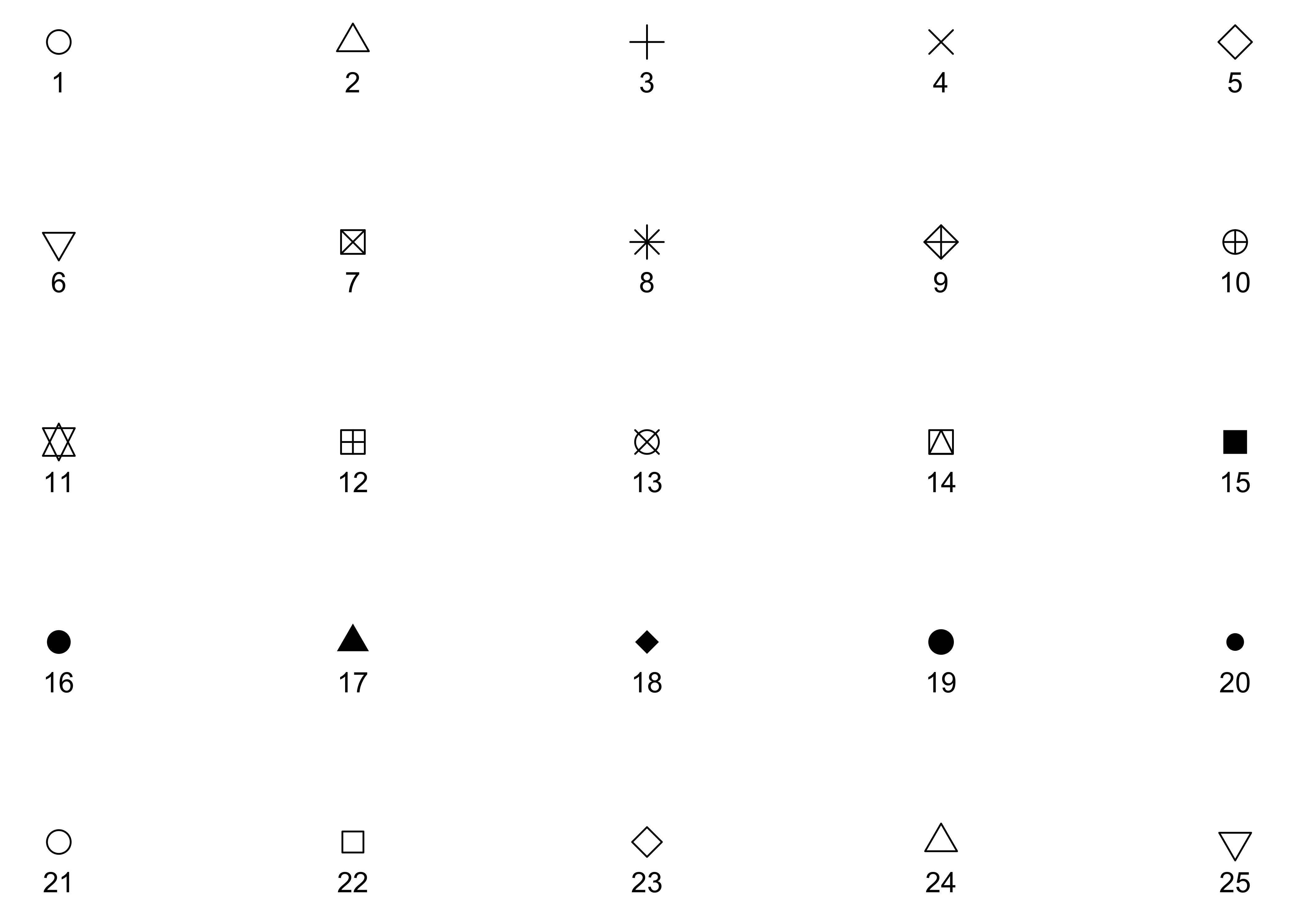

All symbols have a foreground colour, so if we add color = "navy", they all are affected.

s + geom_point(aes(shape = z), size = 4, colour = "blue")  + scale_shape_identity()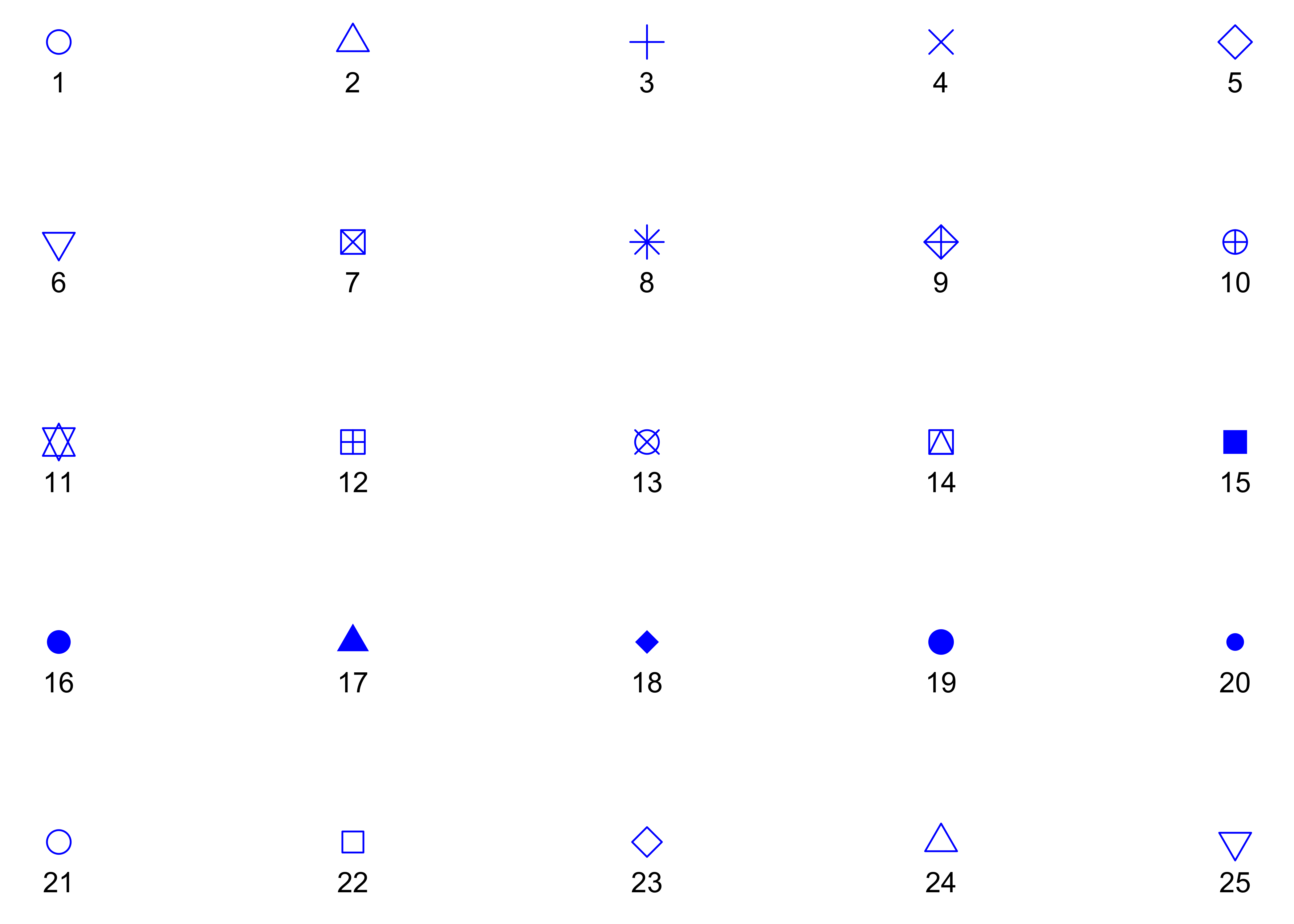

While all symbols have a foreground colour, symbols 21-25 also take a background colour (fill). So if we add fill = "orchid", only the last row of symbols are affected.

s + geom_point(aes(shape = z), size = 4, colour = "blue", fill = "orchid")  + scale_shape_identity()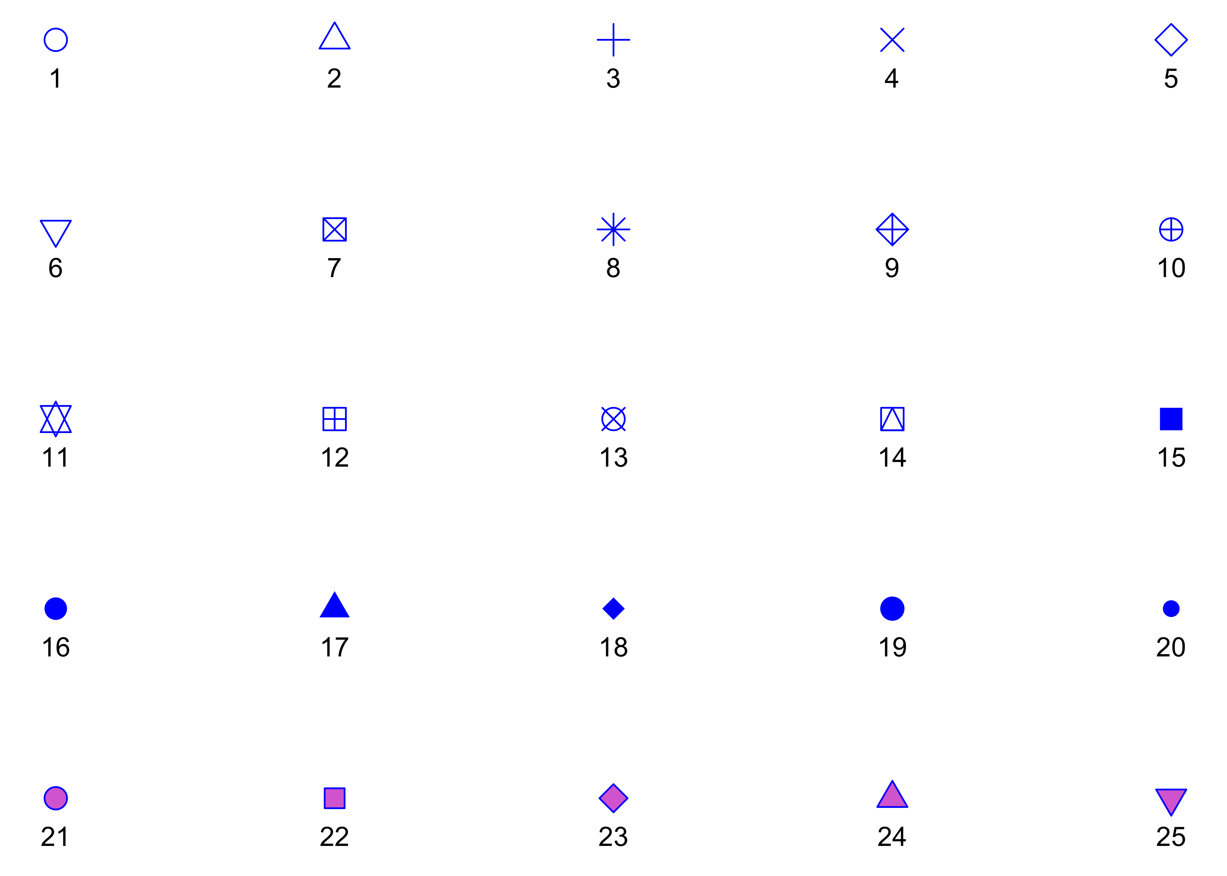

Discrete vs continuous variables

WHAT IS THE DIFFERENCE BETWEEN CATEGORICAL, ORDINAL AND INTERVAL VARIABLES?

In order to use color with your data, most importantly, you need to know if you’re dealing with discrete or continuous variables.

Some Colour Palette Packages in R

We have the following example packages that offer palettes in R:

RColorBrewer
wesanderson
paletteer
colorspace

See Appendix for a detailed graphical analysis of these palette packages.

Colour Palette Types

These palettes can be:

Sequential (type = “seq”) palettes are suited to ordered data that progress from low to high. Lightness steps dominate the look of these schemes, with light colors for low data values to dark colors for high data values. (for numerical data, that are ordered)

Diverging (type = “div”) palettes put equal emphasis on mid-range critical values and extremes at both ends of the data range. The critical class or break in the middle of the legend is emphasized with light colors and low and high extremes are emphasized with dark colors that have contrasting hues.(for numerical data that can be positive or negative, often representing deviations from some norm or baseline)

Qualitative (type = “qual”) palettes do not imply magnitude differences between legend classes, and hues are used to create the primary visual differences between classes. Qualitative schemes are best suited to representing nominal or categorical data. (for qualitative unordered data)

Create a simple set of scatter plots

We will create simple base plots in ggplot and see how we may alter the colour scales using palettes.

names(penguins)

[1] "species"           "island"            "bill_length_mm"   
[4] "bill_depth_mm"     "flipper_length_mm" "body_mass_g"      
[7] "sex"               "year"

p1 <- penguins %>% 
  drop_na() %>% 
  # pipe data into ggplot
  # after removing data rows that have missing ( NA ) values
  ggplot(aes(y = body_mass_g, x = flipper_length_mm, 
           color = species # COLOUR = DISCRETE/QUAL VARIABLE
           )) +
           geom_point() + 
           labs(title = "Default Colours in ggplot", 
                subtitle = "P1: DISCRETE/QUAL Colour Palette")


p2 <- 
penguins %>% 
  drop_na() %>% 
  # pipe the data into ggplot, 
  # after removing data rows that have missing ( NA ) values
  ggplot(aes(y = body_mass_g, x = flipper_length_mm, 
           color = bill_length_mm # COLOUR = CONT/QUANT VARIABLE
           )) +
           geom_point() + 
           labs(title = "Default Colours in ggplot", 
                subtitle = "P2: CONTINUOUS/QUANT Colour Palette")

p1

p2

Note that these use the default colours in R.

Colours for Discrete (QUAL) Variables

The commands below are used to fill colours based on Qualitative Variables:

scale_colour/fill_discrete
scale_colour/fill_brewer # RColorBrewer
….

Now to use these!

Plotting Colours based on Discrete Variables

Discrete n-Colour palettes from `RColorBrewer`

RColorBrewer::brewer.pal.info

ABCDEFGHIJ0123456789

	maxcolors <dbl>	category <chr>	colorblind <lgl>
BrBG	11	div	TRUE
PiYG	11	div	TRUE
PRGn	11	div	TRUE
PuOr	11	div	TRUE
RdBu	11	div	TRUE
RdGy	11	div	FALSE
RdYlBu	11	div	TRUE
RdYlGn	11	div	FALSE
Spectral	11	div	FALSE
Accent	8	qual	FALSE

RColorBrewer::display.brewer.all()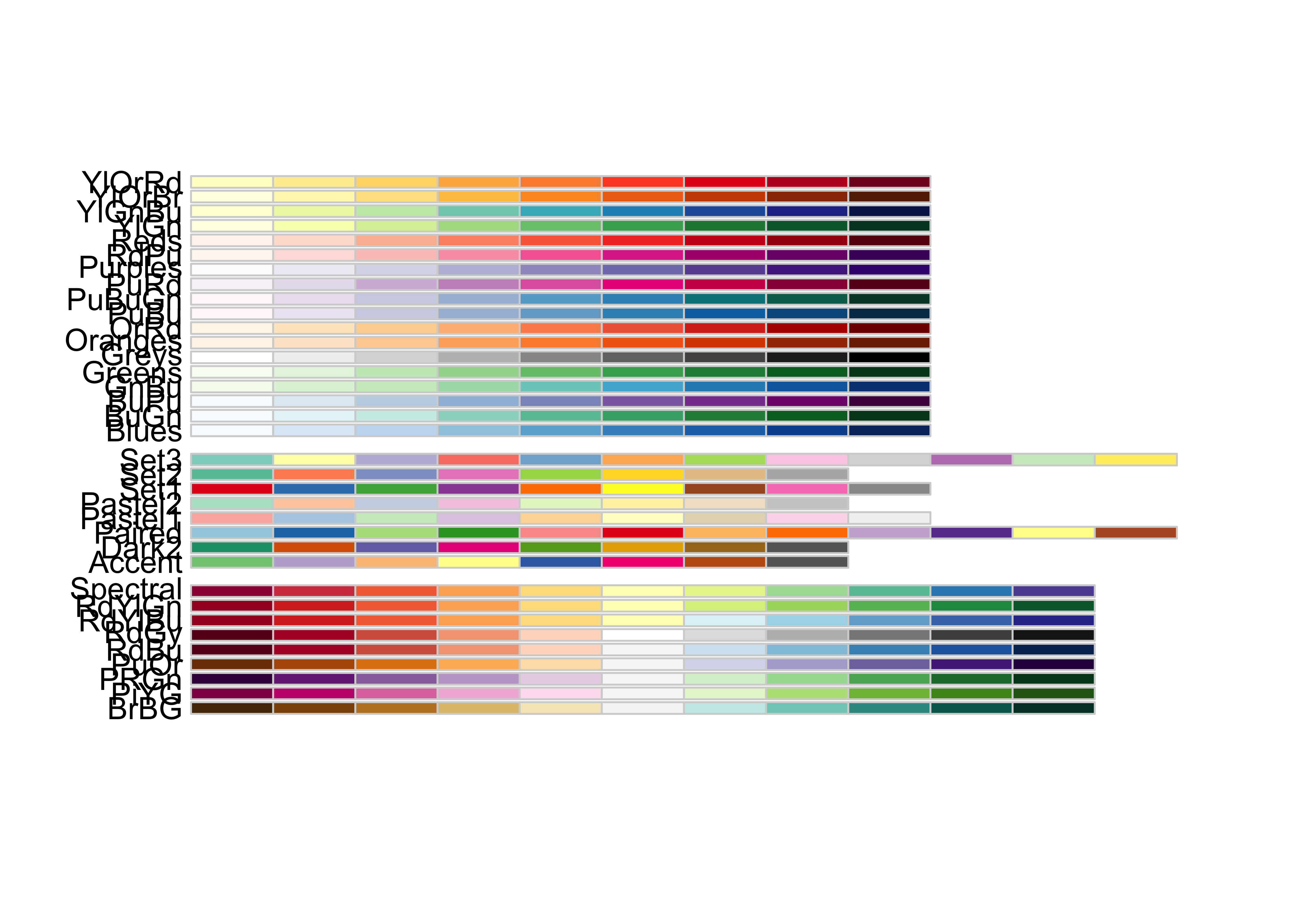

p1 +
  # default palette = "Blues"
  scale_colour_brewer() +
  labs(title = "Brewer Palette = Blues")

p1 +
  scale_color_brewer(palette = "Spectral") +
  labs(title = "Brewer Palette = Spectral")

Discrete Colour scales using `wesanderson` palettes

wesanderson::wes_palettes %>% names()

 [1] "BottleRocket1"     "BottleRocket2"     "Rushmore1"        
 [4] "Rushmore"          "Royal1"            "Royal2"           
 [7] "Zissou1"           "Zissou1Continuous" "Darjeeling1"      
[10] "Darjeeling2"       "Chevalier1"        "FantasticFox1"    
[13] "Moonrise1"         "Moonrise2"         "Moonrise3"        
[16] "Cavalcanti1"       "GrandBudapest1"    "GrandBudapest2"   
[19] "IsleofDogs1"       "IsleofDogs2"       "FrenchDispatch"   
[22] "AsteroidCity1"     "AsteroidCity2"     "AsteroidCity3"

p1 +
  scale_colour_discrete(type = wes_palette(name = "GrandBudapest1",
                                           n = 3)) +
  labs(title = "Wes Anderson Palette: GrandBudapest")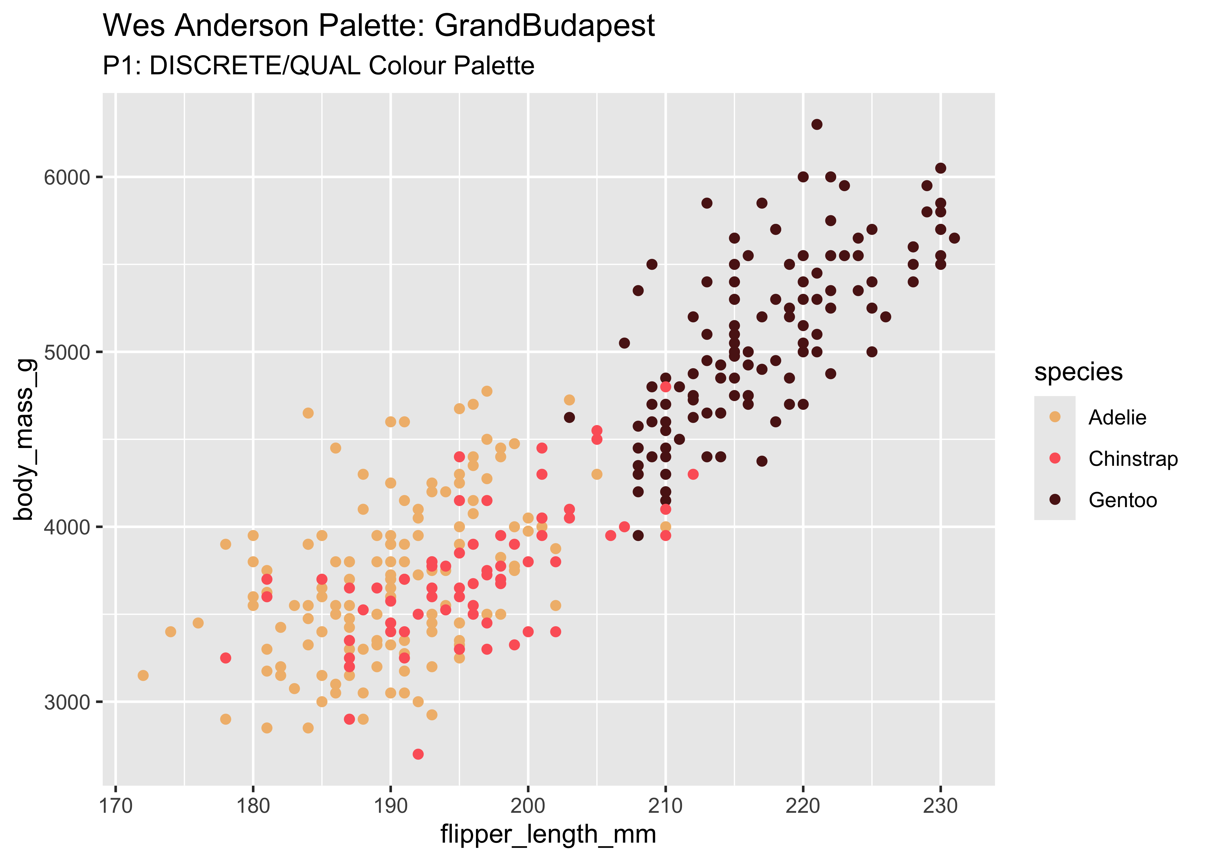

# We can also specify colour codes ourselves with scale_x_discrete.
# Use argument "values" instead of "type"
manual_colours <- c("#afc4b8", "#f1a4b2", "#ffb1e1") 
manual_colours

[1] "#afc4b8" "#f1a4b2" "#ffb1e1"

p1 +
  scale_colour_manual(values =  manual_colours) +
  labs(title = "Manual Colours")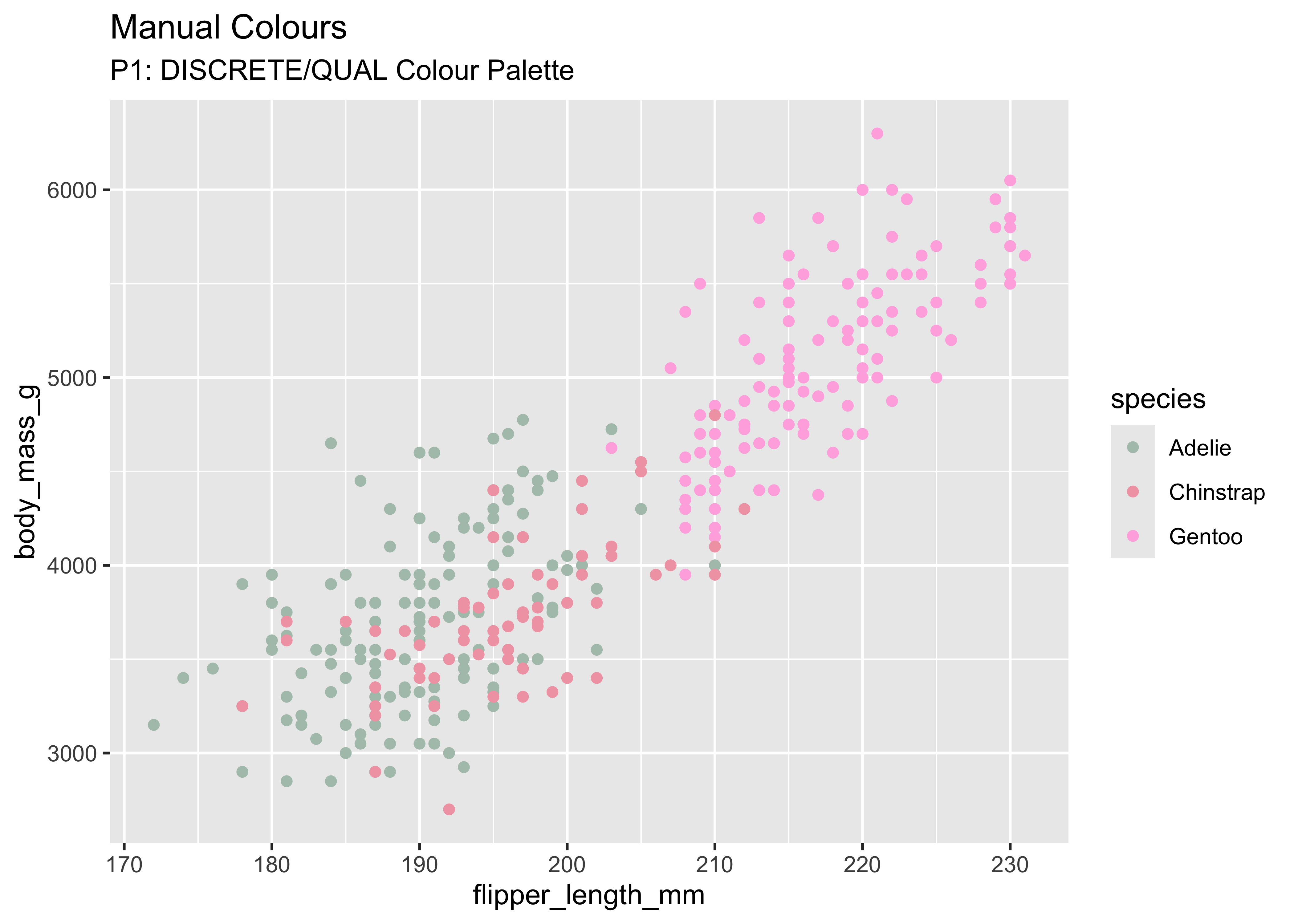

Discrete n-Colour palettes from `RColorBrewer`

# scale_x_brewer() for DISCRETE data
p1 +
  scale_colour_brewer(palette = "Spectral") +
  
  labs(title = "RColorBrewer Palette = Spectral")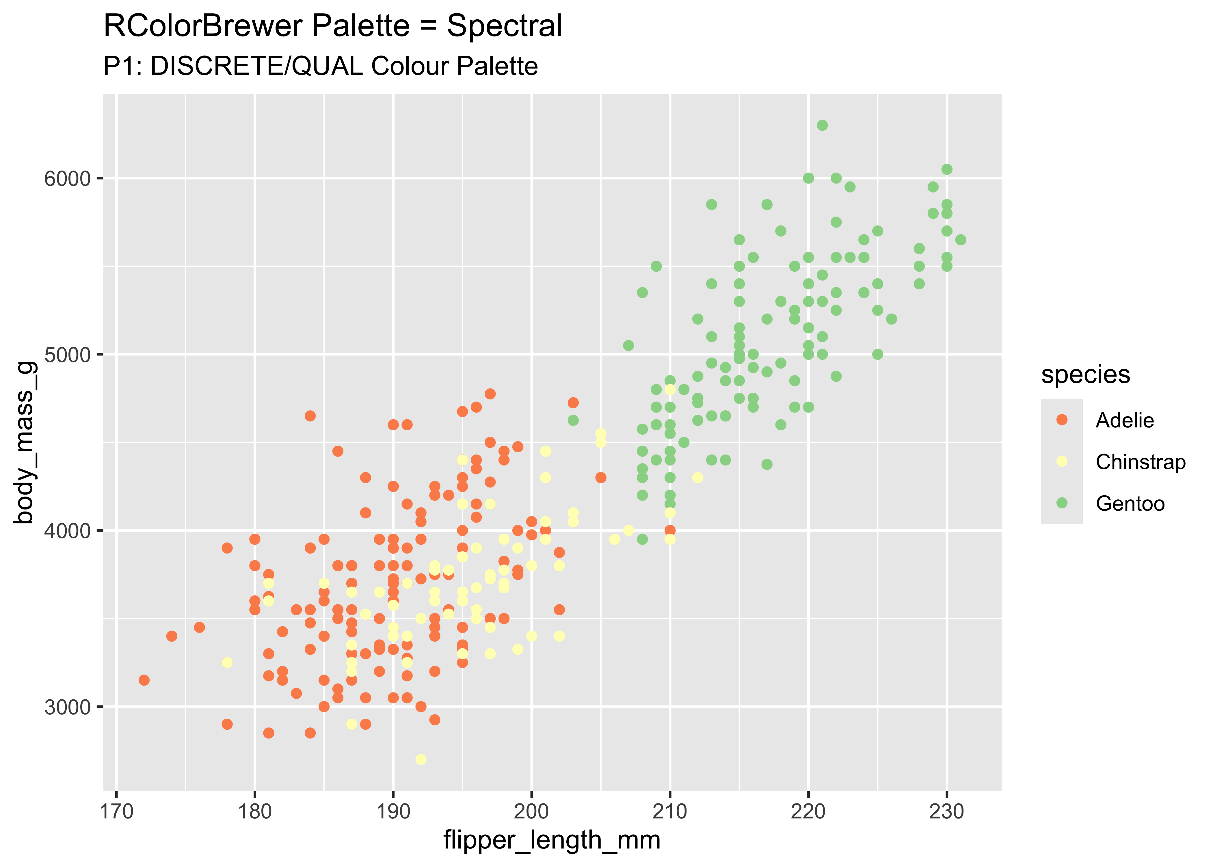

Discrete Colour scales using `paletteer` palettes

palettes_d_names

ABCDEFGHIJ0123456789

package <chr>	palette <chr>	length <int>	type <chr>	novelty <lgl>
awtools	a_palette	8	sequential	TRUE
awtools	ppalette	8	qualitative	TRUE
awtools	bpalette	16	qualitative	TRUE
awtools	gpalette	4	sequential	TRUE
awtools	mpalette	9	qualitative	TRUE
awtools	spalette	6	qualitative	TRUE
basetheme	brutal	10	qualitative	TRUE
basetheme	clean	10	qualitative	TRUE
basetheme	dark	10	qualitative	TRUE
basetheme	deepblue	10	qualitative	TRUE

palettes_dynamic_names

ABCDEFGHIJ0123456789

package <chr>	palette <chr>	length <int>	type <chr>
cartography	blue.pal	20	sequential
cartography	orange.pal	20	sequential
cartography	red.pal	20	sequential
cartography	brown.pal	20	sequential
cartography	green.pal	20	sequential
cartography	purple.pal	20	sequential
cartography	pink.pal	20	sequential
cartography	wine.pal	20	sequential
cartography	grey.pal	20	sequential
cartography	turquoise.pal	20	sequential

paletteer_d("dutchmasters::pearl_earring")

<colors>
#A65141FF #E7CDC2FF #80A0C7FF #394165FF #FCF9F0FF #B1934AFF #DCA258FF #100F14FF #8B9DAFFF #EEDA9DFF #E8DCCFFF

paletteer_dynamic("ggthemes_ptol::qualitative", n = 3)

<colors>
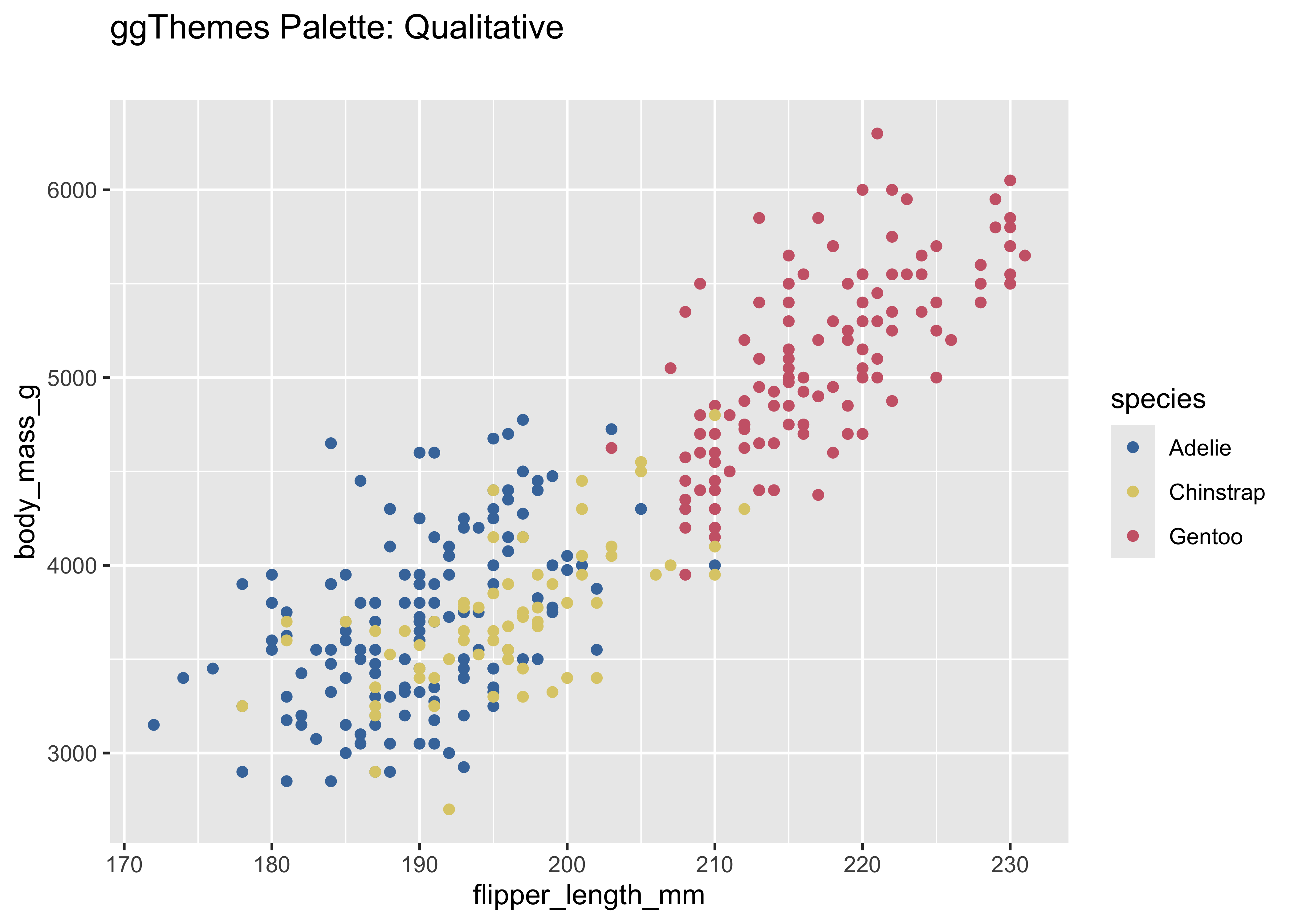
#4477AAFF #DDCC77FF #CC6677FF

p1 +
  scale_colour_paletteer_d("ggthemes_ptol::qualitative", 
                           dynamic = TRUE) +
  
  labs(title = "ggThemes Palette: Qualitative", 
          subtitle = "")

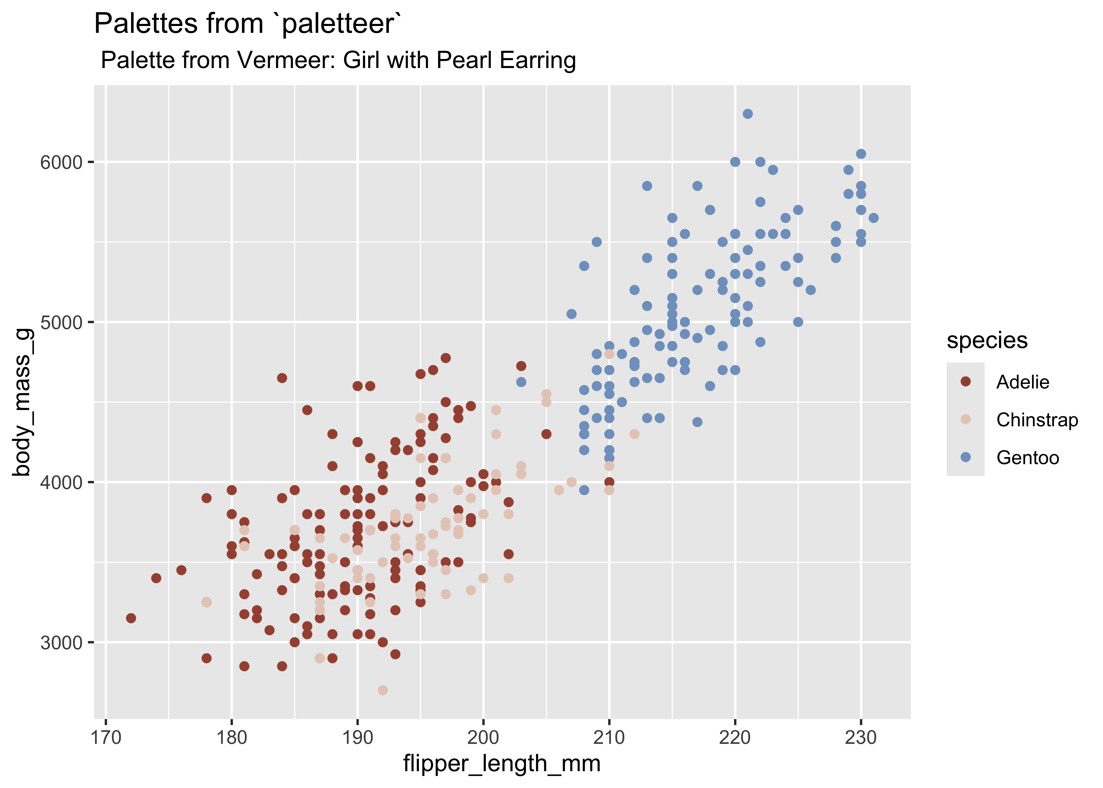
# I like Vermeer's "Girl with the Pearl Earring"!
p1 +
  scale_colour_paletteer_d("dutchmasters::pearl_earring",
                           dynamic = FALSE) +
  
  labs(title = "Palettes from `paletteer`", 
          subtitle = " Palette from Vermeer: Girl with Pearl Earring")

Colours for Continuous (QUANT) Variables

The commands below are used to fill colours based on Quantitative Variables:

scale_colour/fill_gradient (Two colour gradient)
scale_colour/fill_gradient2 (Three colour gradient)
scale_colour/fill_gradientn (Specify Palette, from other packages also, like wesanderson )
scale_colour/fill_distiller (Palettes from RColorBrewer)

Plotting Colours based on Continuous Variables

Continuous Two Colour Gradients

Creates a pallete containing continuous shades between two colours:

p2 +
    scale_color_gradient(
      low = "yellow", # Play with this in the chunk below
      high = "purple") + # Play with this in the chnk below
  
  labs(title = "Two Colour Gradients",
          subtitle = "P2: Continuous 2-Colour Pallete")

Continuous Three Colour Gradients

Sometimes we want a palette this way: a midpoint colour, and colours for the two extremes of a continuous variable:

colour_midpoint <- mean(penguins$bill_length_mm, 
                         na.rm = TRUE) # remove missing values
# Struggled all morning on 22 Aug 2020 to get at this ;-D

# Play with the function: 0/mean/median/mode/max/min

p2 +
  scale_colour_gradient2(
  low = "brown", # Play with this in the chunk below
  mid = "white", # Play with this in the chunk below
  high = "purple", # Play with this in the chunk below
  midpoint = colour_midpoint, # see above
  space = "Lab", # don't mess with this!
  na.value = "grey50")  +
  labs(title = "Three colour continuous gradient", 
          subtitle = "Mid Colour mapped to midpoint of data variable",
          caption = "Colours inspired by my favourite cocker spaniel, Lord Chestnut") # Play with these

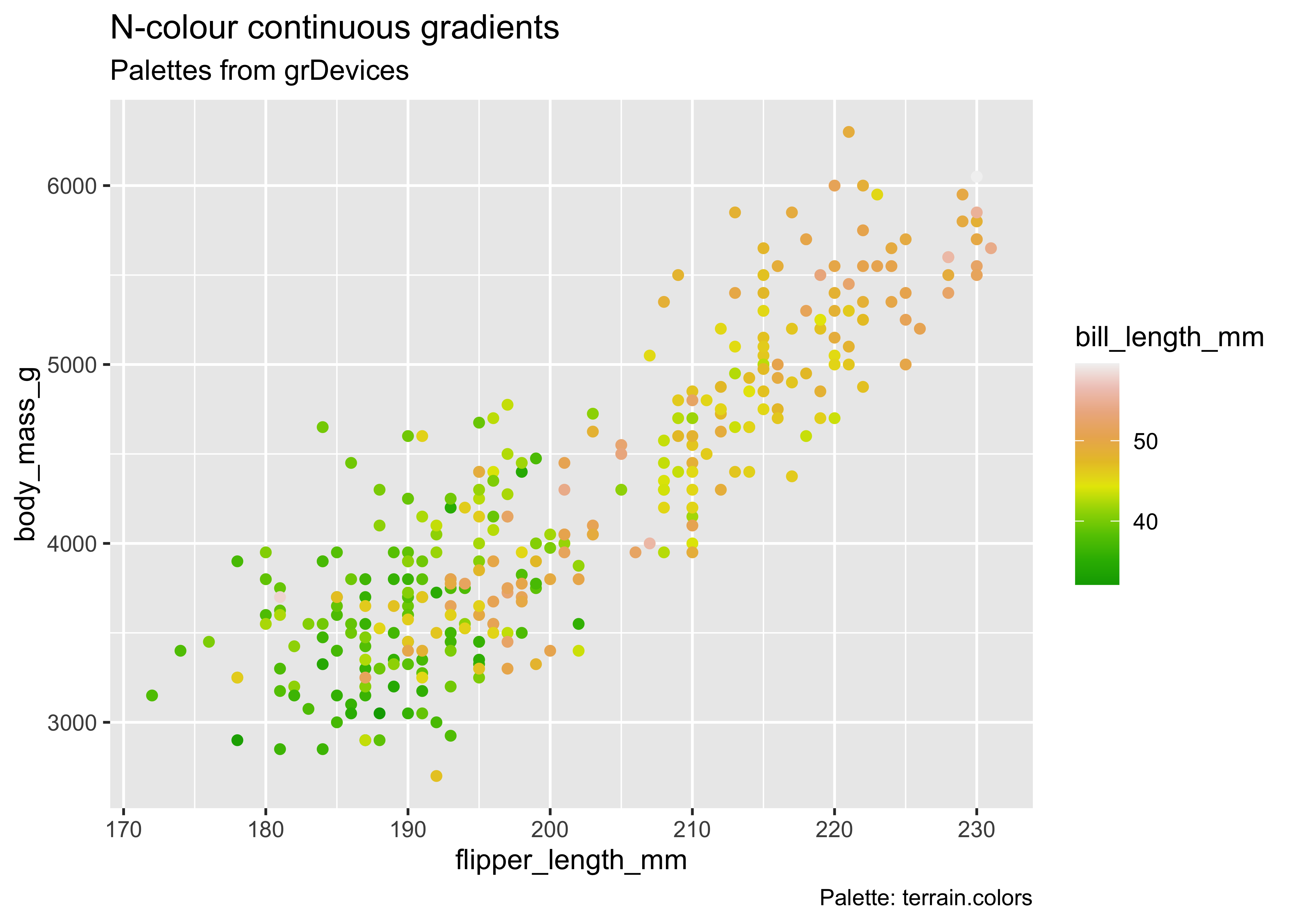
Continuous n-Colour Gradients - `grDevices` package

# grDevices Palettes
p2 +
  scale_colour_gradientn(
    colours = terrain.colors(10)) +
  # Try these:
  # heat.colors() / topo.colors() / cm.colors() / rainbow()
  
  labs(title = "N-colour continuous gradients", 
          subtitle = "Palettes from grDevices",
          caption = "Palette: terrain.colors")

Continuous n-Colour Gradients - `wesanderson` Palettes

wes_palettes

$BottleRocket1
[1] "#A42820" "#5F5647" "#9B110E" "#3F5151" "#4E2A1E" "#550307" "#0C1707"

$BottleRocket2
[1] "#FAD510" "#CB2314" "#273046" "#354823" "#1E1E1E"

$Rushmore1
[1] "#E1BD6D" "#EABE94" "#0B775E" "#35274A" "#F2300F"

$Rushmore
[1] "#E1BD6D" "#EABE94" "#0B775E" "#35274A" "#F2300F"

$Royal1
[1] "#899DA4" "#C93312" "#FAEFD1" "#DC863B"

$Royal2
[1] "#9A8822" "#F5CDB4" "#F8AFA8" "#FDDDA0" "#74A089"

$Zissou1
[1] "#3B9AB2" "#78B7C5" "#EBCC2A" "#E1AF00" "#F21A00"

$Zissou1Continuous
 [1] "#3A9AB2" "#6FB2C1" "#91BAB6" "#A5C2A3" "#BDC881" "#DCCB4E" "#E3B710"
 [8] "#E79805" "#EC7A05" "#EF5703" "#F11B00"

$Darjeeling1
[1] "#FF0000" "#00A08A" "#F2AD00" "#F98400" "#5BBCD6"

$Darjeeling2
[1] "#ECCBAE" "#046C9A" "#D69C4E" "#ABDDDE" "#000000"

$Chevalier1
[1] "#446455" "#FDD262" "#D3DDDC" "#C7B19C"

$FantasticFox1
[1] "#DD8D29" "#E2D200" "#46ACC8" "#E58601" "#B40F20"

$Moonrise1
[1] "#F3DF6C" "#CEAB07" "#D5D5D3" "#24281A"

$Moonrise2
[1] "#798E87" "#C27D38" "#CCC591" "#29211F"

$Moonrise3
[1] "#85D4E3" "#F4B5BD" "#9C964A" "#CDC08C" "#FAD77B"

$Cavalcanti1
[1] "#D8B70A" "#02401B" "#A2A475" "#81A88D" "#972D15"

$GrandBudapest1
[1] "#F1BB7B" "#FD6467" "#5B1A18" "#D67236"

$GrandBudapest2
[1] "#E6A0C4" "#C6CDF7" "#D8A499" "#7294D4"

$IsleofDogs1
[1] "#9986A5" "#79402E" "#CCBA72" "#0F0D0E" "#D9D0D3" "#8D8680"

$IsleofDogs2
[1] "#EAD3BF" "#AA9486" "#B6854D" "#39312F" "#1C1718"

$FrenchDispatch
[1] "#90D4CC" "#BD3027" "#B0AFA2" "#7FC0C6" "#9D9C85"

$AsteroidCity1
[1] "#0A9F9D" "#CEB175" "#E54E21" "#6C8645" "#C18748"

$AsteroidCity2
[1] "#C52E19" "#AC9765" "#54D8B1" "#b67c3b" "#175149" "#AF4E24"

$AsteroidCity3
[1] "#FBA72A" "#D3D4D8" "#CB7A5C" "#5785C1"

names(wes_palettes)

 [1] "BottleRocket1"     "BottleRocket2"     "Rushmore1"        
 [4] "Rushmore"          "Royal1"            "Royal2"           
 [7] "Zissou1"           "Zissou1Continuous" "Darjeeling1"      
[10] "Darjeeling2"       "Chevalier1"        "FantasticFox1"    
[13] "Moonrise1"         "Moonrise2"         "Moonrise3"        
[16] "Cavalcanti1"       "GrandBudapest1"    "GrandBudapest2"   
[19] "IsleofDogs1"       "IsleofDogs2"       "FrenchDispatch"   
[22] "AsteroidCity1"     "AsteroidCity2"     "AsteroidCity3"

p2 +
    scale_colour_gradientn(
      colors = wes_palette(name = "GrandBudapest1", 
                           n = 4), # Keep an eye on "n".
      na.value = "grey") +
  # Try these:
  # "BottleRocket1"  "BottleRocket2"  "Rushmore1"
  # "Rushmore"       "Royal1"         "Royal2"
  # "Zissou1"        "Darjeeling1"    "Darjeeling2"   
  # "Chevalier1"     "FantasticFox1"  "Moonrise1"     
  # "Moonrise2"      "Moonrise3"      "Cavalcanti1"   
  # "GrandBudapest1" "GrandBudapest2" "IsleofDogs1"   
  # "IsleofDogs2"   
  # Keep an eye on "n".
  
  labs(title = "N-colour continuous gradients", 
       subtitle = "Palettes from wesanderson",
       caption = "Palette: GrandBudapest1") # Change this caption based on palette choice

Continuous n-Colour palettes from `RColorBrewer`

Recall Palette types

seq for continuous data mapped to colour
qual for categorical data mapped to colour ( discrete)
div continuous data mapped to colour, that has pos and neg extremes from a middle value

brewer.pal.info

ABCDEFGHIJ0123456789

	maxcolors <dbl>	category <chr>	colorblind <lgl>
BrBG	11	div	TRUE
PiYG	11	div	TRUE
PRGn	11	div	TRUE
PuOr	11	div	TRUE
RdBu	11	div	TRUE
RdGy	11	div	FALSE
RdYlBu	11	div	TRUE
RdYlGn	11	div	FALSE
Spectral	11	div	FALSE
Accent	8	qual	FALSE

# scale_color_distiller() and scale_fill_distiller() 
# are used to apply the ColorBrewer colour scales 
# to continuous data.

p2 +
  scale_colour_distiller(
    palette = "YlGnBu") + # Play with this palette
  
  labs(title = "RColorBrewer Palette")

Continuous Colour scales using `paletteer` palettes

This palette seems to have everything accessible in a simple way! NOTE: In order to access some palettes in paletteer, you may be asked to install other packages. E.g. harrypotter or scico. These need not be brought into your session using library() but are accessed directly by paletteer which is very convenient!!

# What continuous palettes are there in paletteer?
paletteer::palettes_c_names

ABCDEFGHIJ0123456789

package <chr>	palette <chr>	type <chr>
ggthemes	Blue-Green Sequential	sequential
ggthemes	Blue Light	sequential
ggthemes	Orange Light	sequential
ggthemes	Blue	sequential
ggthemes	Orange	sequential
ggthemes	Green	sequential
ggthemes	Red	sequential
ggthemes	Purple	sequential
ggthemes	Brown	sequential
ggthemes	Gray	sequential

OK, one of the Games of Thrones Palettes, and Harry Potter!

p2 +
  # scale_colour_paletteer_c("gameofthrones::jon_snow") +
  # Temporarily not available in paletteer?
  
  scale_colour_paletteer_c(`"harrypotter::dracomalfoy"`) +
  labs(title = "Using Paletteer",
       subtitle = "Continuous Palette-Hary Potter: Draco Malfoy",
       caption = "Oh you awful Srishti people...")

Error in `gen_fun()`:
! The package "harrypotter" is required.

  # Harry Potter Gryffindor Palette.
  # Will ask for `harrypotter` package to be installed. Say yes!
  p2 +
  scale_colour_paletteer_c("harrypotter::gryffindor") +
  labs(title = "Using Paletteer",
       subtitle = "Continuous Palette-Harry Potter: Gryffindor")

Error in `gen_fun()`:
! The package "harrypotter" is required.

Setting up R Packages

Introduction

Goals

Pedagogical Note

Data

Colour vs fill aesthetic

Discrete vs continuous variables

Some Colour Palette Packages in R

Colour Palette Types

Create a simple set of scatter plots

Colours for Discrete (QUAL) Variables

Plotting Colours based on Discrete Variables

Discrete n-Colour palettes from RColorBrewer

Discrete Colour scales using wesanderson palettes

Discrete n-Colour palettes from RColorBrewer

Discrete Colour scales using paletteer palettes

Colours for Continuous (QUANT) Variables

Plotting Colours based on Continuous Variables

Continuous Two Colour Gradients

Continuous Three Colour Gradients

Continuous n-Colour Gradients - grDevices package

Continuous n-Colour Gradients - wesanderson Palettes

Continuous n-Colour palettes from RColorBrewer

Continuous Colour scales using paletteer palettes

Discrete n-Colour palettes from `RColorBrewer`

Discrete Colour scales using `wesanderson` palettes

Discrete n-Colour palettes from `RColorBrewer`

Discrete Colour scales using `paletteer` palettes

Continuous n-Colour Gradients - `grDevices` package

Continuous n-Colour Gradients - `wesanderson` Palettes

Continuous n-Colour palettes from `RColorBrewer`

Continuous Colour scales using `paletteer` palettes